MIT 6.046 - Design and Analysis of Algorithms

6.046 is described by Eric Demaine as the final undergraduate algorithms class, with more advanced and more specialized algorithms classes being at the graduate level.  I've had my eye on the advanced data structures and advanced algorithms classes for a while, and this class is a fundamental prerequisite for those.  Now, being that it's my MO to totally overdo it, naturally I had to find overlapping classes from some of my other favorite providers and watch everything.  Had I limited this to one overlapping class it probably wouldn't have been that bad... but I found three other classes: Berkeley CS170, Georgia Tech CS6505, and Stanford CS261.  All four classes are what I would call "intermediate" level algorithms courses, with significant overlap in concepts covered:

I probably would have been done a month ago if I hadn't gone so crazy with watching everyone's lectures...

Course Resources

MIT OpenCourseware Site
MIT Stellar Course Website
MIT Lecture Playlist on YouTube
Textbook: CLRS

Full Reading List [personal recommendation]:

• Lecture 1: section 16.1
• Lecture 2: section 9.3 [chapter 9]
• Recitation 1: - [chapter 4]
• Lecture 3: chapter 30
• Recitation 2: chapter 18
• Lecture 4: chapter 20
• Recitation 3: chapter 17
• Lecture 5: chapter 17
• Lecture 6: chapter 7
• Recitation 4: -
• Lecture 7: -
• Lecture 8: section 11.5
• Recitation 5: - [chapter 15]
• Lecture 9: chapter 14
• Lecture 10: chapter 15
• Lecture 11: chapter 15
• Lecture 12: chapter 16
• Recitation 6: -
• Lecture 13: chapter 26
• Lecture 14: section 26.3
• Recitation 7: -
• Lecture 15: chapter 29
• Lecture 16: chapter 34
• Recitation 8: -
• Lecture 17: chapter 35
• Recitation 9-11: -
• Lecture 18-24: -

Complementary Courses (Cover much of the same material):

• Georgia Tech CS6505, Computability, Complexity & Algorithms (call it GTech)
• UC Berkeley CS170, Efficient Algorithms and Intractable Problems: Website. Lectures (2015). Lectures (2012)
• Stanford CS261, A Second Course In Algorithms: Website, Lectures

Week 1: Divide and Conquer

Readings this week are sections 16.1 (interval scheduling problem) and 9.3 (efficient order statistics, i.e. median and ith element algorithms).  I just went ahead and read the whole chapter 9 for context, it wasn't bad.  Lecture 1 covered the obligatory logistical info before digging right into the interval problem.

The premise for the interval scheduling problem is that we have n requests for some resource, and each request has a start and end time, such that s < f, i.e. no zero length requests.  We have to pick the maximum sized subset of these requests.  There is an efficient Greedy solution to this problem that follows this template:

1. Pick interval with some rule
2. Eliminate all incompatible (overlapping) intervals from set
3. Repeat one and two until all intervals either eliminated or added to solution

The devil with the Greedy approach is picking the right rule for step 1.  Several obvious picks (smallest interval first, earliest start time first, least number of conflicts first) all have a counter example.  The correct solution is to choose the interval with the earliest finish time first.  This always leads to a correct solution.

Now, when we add weights to the interval, and try to maximize the total value of these weights, Greedy will no longer work.  We need to use a DP approach to get a correct answer.  The approach discussed in lecture chooses each interval as a potential first, the recurses on the set of intervals compatible with the chosen interval, memoizing as it goes.  Because each subproblem runs in linear time, this algorithm runs in O(n²).  Introducing the notion of separate machines to process the requests makes the problem NP-Complete.

Recitation 1 takes a second look at this problem. By sorting the intervals on their starting time, we can reduce the subproblems at each step from n to 2.  We subsequently end up with an O(n lg n) solution.

Lecture 2 covers a divide and conquer convex hull algorithm and median finding.  The brute force approach to convex hull involves taking a half plane through two points, and just testing if all the other points fall on one side of the half plane.  When all the points are on one side of the line segment, that segment is part of the hull.  This algorithm is cubic, since there are n² segments to test, and testing requires O(n) work.

Divide and conquer can be applied to this problem, recursively dividing the points in half (they demonstrate using the x coordinates).  Once he problem is small enough, just run the brute force algorithm.  The interesting bit is in merging the two subproblems.  Using a simplistic rule like "connect the points from each side with highest/lowest y value" can lead to incorrect results.  The correct solution is to use a "two finger" algorithm that circles around each hull, testing the y intercept of the connecting segments.  The line with the maximum y intercept is the correct top tangent, and the segment with the lowest intercept is the bottom tangent.  To return the correct set of segments, simply start at one of the tangent points and circle around clockwise.

The divide and conquer approach to "order statistics", which include min, max, median, and "rank", or ith element, is covered in chapter 9 of CLRS.  Srini points out that while convex hull is interesting in the merge portion, median finding is interesting in the divide portion of the problem.  The approach to the problem is very much like quick sort:  the array is partitioned around a pivot.  The big difference from quicksort is that you only recurse on one side of the partition.  Like quicksort, if we are very unlucky with our pivots we can do a lot of repeated work and end up with an O(n²) algorithm.

The reading (section 9.3) covers an algorithm that is clever in the way it picks the pivot to guarantee a good pivot and thus an O(n) worst case algorithm.  The array is divided into n/5 groups of 5 elements.  Each group is sorted, and the median identified.  We then identify the median of these medians, and use that as the pivot.  This works because it ensures that a non-trivial portion of the values are in each partition (that is, the partitions are balanced).

The recitation also reviews Master Theorem, using Strassen's Algorithm for matrix multiplication as a motivating example.  We can use the Master Theorem technique when our recurrence relations takes the form:

T(n) = aT(n/b) + f(n)

a is the branching factor, and b determines how small each subproblem gets.  a ≥ 1, and b > 1.

There are three cases (please forgive the terrible typography...):

1. f(n) = O(n^c) where c < log_b(a).  This is the "geometric sequence" recurrence, where most of the work is being done in the leaves.  The result is Θ(n^log_b(a)).  
2. f(n) = Θ(n^c * log^k(n)) where c = log_b(a).  In this case, the "divide" portion and the "merge" portion are the same size.  Results in Θ(n^c * log^k+1(n))
3. f(n) = Ω(n^c) where c > log_b(a).  This is the top heavy recurrence, where the work of f(n) dominates.  Result is Θ(f(n)).

I'll admit I was pretty rusty with recurrence analysis (it's been a while since 6.006, and even then I wasn't exactly a master).  Chapter 4 in CLRS provides a pretty robust discussion of not only the master theorem, but substitution and recurrence tree approaches as well.  Since master theorem is only applicable in certain cases, the other two approaches will be valuable tools as well (guess I have some more reading to do...)

The first 4 lectures of CS170 (Spring 2015) cover some of the same ideas.  I will say I like the videos for 6.046 better than the CS170 videos (the bits where they write on the touchscreen can be hard to see).  They cover the Karatsuba algorithm for multiplication, Strassen matrix multiplication, master theorem, merge sort, and median finding.

Week 2: FFT, B-trees

According to the wikipedia entry for the Fast Fourier Transform, Fourier analysis is a process that "converts a signal from it's original domain... to a representation in the frequency domain".   This week dives into how the FFT uses a divide and conquer approach to reduce the straightforward O(n²) computation down to O(n lg n).  I'll be the first to admit that I struggled with this algorithm.  CLRS devotes a whole chapter to the subject and while I "finished" it, it didn't click.  Luckily, Demaine does a great job walking through the concepts involved, and supplementing with CS170 Lecture 5 and Lecture 6, and the GTech Lesson on FFT, helped me (mostly) wrap my head around what is happening.

The motivation behind all three sets of lectures is the need to do fast polynomial multiplication.  Doing this long form (as we learned in early algebra), multiplying polynomials A and B is roughly quadratic in complexity (we have to multiply every term in A with every term in B).   This is equivalent to doing a convolution of the two sets of terms: reverse B, and "slide" it under A, multiplying the individual terms and adding them up:

Good thing I have WolframAlpha to check my work...

Above is the coefficient representation of a polynomial.  It is also possible to represent a polynomial as a series of points.  For a polynomial of degree 1 (a line), we need two distinct points to define the unique polynomial.  Degree 2 needs three points, generally a polynomial of degree d needs d  + 1 points to define it.  What is convenient about this representation is that multiplying two polynomials which points defined at the same x coordinates is just a point-wise operation that takes linear time.  The problem is that evaluating arbitrary points requires interpolating the polynomial, which takes quadratic time.  An evaluation in coefficient form takes linear time.  So the trick is to efficiently convert between the two representations, which is where the FFT comes in.

The "divide" portion of the FFT splits the polynomial into "even" and "odd" factors, so

1 + 2x + x² + 2x³

becomes

1 + x²     and      2x + 2x³

we then factor out an x from the odd side to get:

1 + x²     and      x(2 + 2x²)

This sets us up to reduce the degree of each polynomial, if we substitute y for x²:

1 + y     and      x(2 + 2y)

This, by itself, isn't enough though.  When we work the recurrence, we have n points representing the polynomial.  When we square these values, with real numbers, we still have the same number of terms at each level of the recursion, which leaves us with an algorithm that is still quadratic.  What we need is a set of points that are collapsing when squared.  This is where we get the complex numbers and the nth roots of unity.

A "root of unity" is just a fancy way of saying a "root of one".  The square roots of one are 1 and -1.  The square roots of -1 are i and -i.  And so on.  Erik Demaine gives a very good geometric explanation of the roots of unity (which was reinforced in the other lectures).  The short and long of it is that when you takes the squares of the 8 8th roots of unity, you get the 4 4th roots of unity, then the 2 2nd roots of unity, then 1.  So the set of points we are evaluating gets smaller, leading to an n lg n complexity. (I've glossed over it a bit here, this is just the gist of it).

The actual "conversion" between coefficient and sample space is done by multiplying the vector A of coefficients by the Vandermonde matrix V, a process called the Discrete Fourier Transform, or DFT.  Going in the opposite direction requires multiplying the sample vector A* by the inverse of V.  Using the Vandermonde matrix of the inverse roots of unity and dividing by n is equivalent to using the inverse of V.  While I'm not exactly primed to go implement FFT in software anytime soon, I think I can at least follow the algorithm now without my eyes glazing over.

Recitation 2 is a short treatment on B-trees.  It seems kind of out of place, but maybe it was just mean to prime us for van Emde Boas trees next week...

Week 3: van Emde Boas Trees

Lecture 4 follows chapter 20 in CLRS pretty much point by point.  vEB trees are also touched on in the advanced data structures class (lecture 11) and the Harvard advanced algorithms class (lecture 1), both of which offer a similar perspective.  The 6.046 lecture is a bit more methodical, though, so is probably still the best place to start.

So to begin thinking about vEB trees, we start with a set S represented as a bit vector.  This bit vector is size u, where u is the size of the universe of possible values.  So if the domain of our set is 32 bit integers, it would have about 4 billion entries.  Insert and delete are O(1), since all we are doing is indexing into the array (at S[n]) and flipping the bit.  But successor and predecessor are slow, O(u).  If the first and last bits are set and we call successor(S, 0), we have to traverse the entire array to find the value at S[u-1].

As we work to improve our runtime, we gradually move closer to the vEB data structure.  First we put a full binary tree over top of our array (we assume u is size 2 raised to power of two).  The inner nodes are the OR of their two children.  We can do a binary search like query within this tree structure by using two components of this bit vector + tree structure.  Firstly, we divide the bit vector into √u "clusters" of size √u.  If we don't find our successor in our cluster, then we look halfway up the tree to the "summary vector", which is also of size √u (since we are restricting u size domain).  We find the next non-empty cluster, then find the minimum element in that cluster.

The green arrows trace the search path of successor(0)

Because successor looks at, at most, 3√u, the complexity of successor at this point is O(√u), which is asymptotically worse than just using a BST (which gives us O(lg n) complexity).  This is just the first step, though.  Once we are reducing the problem size by square root recursively, we'll be able to achieve a complexity of O(lg lg u), which for most reasonable size u is better than lg n.

One concept that will become important when we start working with the recursive version of the data structure is the way in which we represent the inserted numbers.  In the above example, a u=16 number can be represented with 4 bits.  While we can calculate the cluster a number belongs in, and the slot in the cluster it occupies, with arithmetic operations, it is actually much more performant to use bit operations to split the number into high and low order bits.  Observe that 15 is 1111 in binary, with the high bits = 3 (11) and the low bits = 3 (11), corresponding to the cluster index, and the index within that cluster.  9 (1001) occupies cluster 2 (10) at position 1 (01).  And so on.

For our recursive data structure, we want the summary and clusters to be the same type of structure, but √u the size.  We also want to augment our data structure with the min and max values (this is important to optimize our runtime later).  I'm also assuming we store the universe size as a field.  The VEB should look something like this:

class VEB{
 int u;
 Integer min;
 Integer max;
 VEB summary;
 VEB[] cluster;
}

Pictorially, it should look a bit like this (like CLRS, treating u == 2 as a base case).  Sorry for the teeny print:

Depth of the tree is O(lg lg u)

Demaine (and the book) walk though several suboptimal ways of implementing successor and insert that result in run times worse than lg lg u.  Getting good performance rests on a couple clever tweaks:

• Recursive functions (insert, successor, delete) can only recurse once. 
• When we insert into an empty cluster, we also have to insert into the summary.  The trick here is that when we insert into an empty cluster, we just set the min and max and do not recurse.  So when we insert into summary, that means the cluster is new (empty) and inserting into it is cheap.
• When we look up successor, we know it is either in our cluster, or the min value of another cluster.  Only one recursive lookup will succeed, so we store the max and use it to determine which recursive call to make.  When we find the right cluster in summary, getting the min value is cheap.
• Because the minimum value is not stored recursively, it gives us a cheap way to check if a cluster is empty (which helps with delete).

Week 4: Amortized Analysis

Amortized analysis is a way of thinking about an algorithm's complexity that can give us tighter bounds for worst case run time.  A classic example is array doubling in dynamic arrays (like ArrayList).  We have an array with capacity n.  When this capacity is reached, the next insert will trigger a array resize (often the new size is 2n, but any multiplicative factor will work).  The items from the old array are copied to the new one, an operation that takes O(n) time.  This may (incorrectly) lead us to conclude that m operations requires O(mn) time, but this fails to take into consideration how often the O(n) doubling operation occurs.  Because an array is half full after a doubling, it takes n/2 additional inserts to trigger the next doubling.  Because only a single O(n) operation occurs for every O(n) inserts, each individual operation is still O(1).  This is the basic intuition (I've glossed over it a bit).

In addition to the lecture by Demaine, there are lectures by Jonathan Shewchuk (Berkeley 61B, 2008, lecture 35) and Charles Leiserson (6.046, 2005) that cover the same material (for the most part).

There are several ways of doing amortized analysis:

Aggregate method.  Shewchuk calls this the "average method".  Basically, you tally up how much it costs to do the entire operation, and you divide that by the number of operations to give you the running time per operation.

Accounting method.  Each operation "pays" a certain amount per operation.  The difference between the actual cost and payment can be "banked" to help pay for a later, more expensive operation.  One key to this method is that the "bank" balance can never be negative.  If it's negative, it means the cost is too low, and the amortized cost is not an upper bound.  I think Shewchuk's exposition on this one is a little bit better than Demaine's, but they are both good.

Charging method.  This one only appears in Demaine's lecture, and seems to be a variation on the accounting method.  The intuition is that instead of building up a bank account, we can go back and "charge" a previous operation when we have an expensive operation.  The keys here are that we can only go backward in time, and we can only "charge" an operation once.

Potential method.  This method is analogous to the physics concept of "potential energy".  For me, this was one of the rare occasions when the book was the resource that helped me "get it" (usually I read something in the book and have to watch the lecture again for it all to "come together").  The "potential" of a data structure is basically the same as the "bank account" from the accounting method.  Like the bank account, the potential needs to be non-negative.  The change in the potential function between operations tells us if an operation saved work (added potential) or pulled work out.

Week 5: Randomized Algorithms

GTech unit on Randomized Algorithms.

This unit looks at algorithms for which random chance plays some sort of role.  The role that randomness plays in the algorithms can vary.  Some algorithms can be made very efficient, such as
Freivalds' algorithm, which uses randomization to verify the result of a matrix multiplication.  This algorithm uses sampling to achieve a runtime of O(n²), however it is not guaranteed to be correct.  This class of randomized algorithm is called a Monte Carlo algorithm, because it is always fast, but may not be correct.  Contrast this with randomized quicksort, which will always return a correctly sorted list, and will usually run in O(n lg n), but it may run in O(n²) in the worst case (albeit with low probability.  Thus quicksort is an example of a Las Vegas algorithm, which is always correct, but may not be fast.  An class of randomized algorithms that is mentioned but not really expanded on is Atlantic City algorithms, which are not guaranteed to be fast or correct.  Honestly I thought the last one was a joke until I googled it.

Because there is an element of chance involved in these algorithms, analyzing their runtimes is more involved, and generally requires looking at expectations.  Here I'm referring to expectation from a probabilistic standpoint.  Most of the probability speak in these lectures wasn't too bad (especially if you've seen something like 6.008... yikes!).  Although in Recitation he was doing some calculus that I didn't quite follow...

I thought the discussion on the Skip List was very interesting.  A skip list is basically a stack of linked lists.  When an item is inserted into the bottom layer, a coin is flipped to see if it should be added to the layer above.  This "coin flip" is repeated until a negative result is received.  In my illustration below, I've added negative and positive infinity at either end of the list to denote that the first and last items to not necessarily have to extend to the top layer... I was just following Srini's example.

Searches start in the top layer.  If the next element in that layer is above the target value, we drop to the next list down, until we are in the bottom layer and can determine where an element is (or should be).  When we delete an element, it must be deleted from every list.

The last 6.046 lecture on randomization dealt with hashing.  While 6.006 kind of hand waves the analysis (according to Demaine, anyway), in that it assumes "simple uniform hashing", here we assume this is not actually a reasonable assumption, and instead use probabilistic analysis to give it a more robust treatment.  The first half of Lecture 3 from CS170 covers hashing as well.

The underlying problem with the "simple uniform hashing" assumption is that it presumes that the keys being hashed are random, which is why it isn't a reasonable assumption.  We shouldn't make assumptions about our inputs.  Instead, we should ensure that, for any input, we can achieve a good worst case run time.  The way this is accomplished with hashing is through the use of a Universal Hash Family.

A universal hash family is a collection of hash functions.  When we created our hashed data structure, we select a hash function at random.  While this sounds excessively abstract (or at least it did to me at first), all this really means is that we accept one or more hash variables at random, which we then use to permute a hash value from the input key (a process that generally involves a modulo operation and one or more prime numbers).  By choosing our hash variables at random, we can achieve the same run time as the random key model, without the silly assumptions about our input.

Demaine goes into great detail on the analysis of universal hashing and why it works.  He looks at two universal hash families (i.e. hash equations that operate with randomly selected variables).  One is a dot product hash, which treats the key as a vector and finds the dot product of the key with random vector a, all mod m (m is table size, and prime).  There are further assumptions about the what the vectors and the universe look like (there is a logarithmic relationship between m and the vectors).  I thought a simpler universal hash function was the equations h(k) = [(a * k + b) mod p] mod m, where a and b are selected uniformly at random and p is a prime number larger than m.

The last bit on hashing dealt with "perfect hashing".  With a static data structure (no inserts or deletes), we can build a hash table that has no collisions (sort of).  The first step is to build a hash table the way we normally would (with collisions in a linked list).  Only instead of a list of objects hashing to the same bucket, we use a second hash table.  This second hash table is the length of the number of keys squared (so if we have three keys, we have a table of size 9).  Because of the birthday paradox, we should be able to map the keys without collisions with a probability of at least 1/2.  If there is a collision, we recreate the bucket with a different hash function.  If any of the buckets are too big (creating a non-linear space tree), then the top level of the map get's redone with a different hash function.  Overall this will give us O(1) lookup and O(n) space, with a polynomial run time for creation.

Week 6: Dynamic Programming, Augmentation

GTech unit on Dynamic Programming (edit distance, chain matrix multiplication, all pairs shortest paths, transitive closure).

CS170 Lectures 14 (longest increasing sub-sequence, gambling strategy, edit distance), 15 (knapsack, all pair shortest path), 16 (min triangulation, traveling salesman), 17 (largest independent set)

Tushar Roy - Dynamic Programming videos

Augmentation sort of gets awkwardly lumped in here because I really didn't have anywhere else to put it.  The idea with augmentation is that we have some function defined for every node in a tree, call it node.f().  If that node is well behaved (can be calculated in O(1) based on the node, it's children, and the children's values for function f), then this augmentation won't affect our asymptotic running time.  Size and height are common functions facilitated with augmentation.  When Erik started talking about "order statistics" it sounded real familiar... because we looked at it in the unit on divide and conquer.  Where that was an O(n) method, we want to use tree augmentation to get an O(lg n) run time.  This is easily accomplished by storing subtree sizes.

6.046, CS170, and GTech all dedicate a significant portion of time to Dynamic Programming.  The discussion of the technique is fairly similar in all three:  recursively divide the problem into smaller problems, and "remember" previous calculations to turn exponential algorithms into polynomial (or at least pseudo-polynomial) solutions.  All three courses make extensive use of specific problem examples to illustrate DP, but I think the book actually does the best job of explicitly characterizing the qualities of a DP algorithm.

The two defining characteristics of a DP problems are optimal substructure and overlapping subproblems.  Having optimal substructure means that finding the optimal solution for a given problem means finding the optimal solution for it's subproblems.  This is similar to divide and conquer in a way:  the problem is broken into smaller pieces, and these subproblems are then solved optimally.  Where DP is different than divide and conquer, however, is that the subproblems in DP overlap.  While solving a given problem, we will often see the same subproblems repeated (think of the naive version of Fibonacci, where the low order Fib numbers are calculated over and over and over again).  The solution is to solve problems once and "remember" the result.

One way of reusing calculation is through the use of "memoization", basically saving calculated results to an array or hash table.  The algorithm tries to "look up" an answer before doing a calculation.  Used in conjunction with recursion, this is called "top-down" DP.

Alternatively, the subproblems can be arranged as a DAG, and calculated in reverse topological order.  What this basically means is we calculate all the smaller subproblems before we attempt to calculate the larger subproblems that depend on them, working our way through the graph of subproblems until we've solved the original problem.  Often, "solving" the problem will yield an optimized value but not the actual solution (see the Rod Cutting example in the book), but most of the problems demonstrated require very little auxiliary information in order to reconstruct the optimal solution.

Erik's "five easy steps to Dynamic Programming" are worth mentioning:

• what are the subproblems?
• what am I guessing?
• write a recurrence
• check that the constraint graph is acyclic (topological ordering)
• solve original problem

The book lays out a four step sequence, which differs from Erik's version (mostly a matter of emphasis I think):

• Characterize optimal solution
• Recursively define value of optimal solution
• Compute value of optimal solution
• Construct an optimal solution from computed information

The point is that you break your problem into smaller problems, solve those smaller problems ("guessing" basically determines how much work is required to solve a subproblem and thus plays a large role in asymptotic analysis), calculating an optimal value, and (optionally) calculating the optimal solution.  To illustrate the difference between the optimal value and optimal solution, think of the rod cutting problem.  The optimal value gives us the maximum amount of revenue we can get from a given length of rod, whereas the optimal solution actually gives us the cut lengths.

I watched Tushar's tutorial videos while studying for my Google interview, and found them to be very well done.  They make for a good complement to all the examples covered in the university courses.  6.046 covers all-pairs shortest path (Floyd-Warshall and Johnson's algorithm), longest palindromic subsequence, optimal weighted BST, coin picking game (similar to minimax), block stacking, and up-left robot grid paths (lectures 10 and 11, and recitation 5).  CLRS uses rod cutting, matrix chain multiplication, longest common subsequence, and optimal BST.  HackerRank has about a zillion DP problems...

Week 7: Graph and Greedy Algorithms

CS170 Lectures 7 (graphs review, DFS, edge types), 8 (DAGs, connectivity), 9 (BFS, Dijkstra), 10 (Bellman-Ford, MST), 11 (the cut property, Kruskal, Union-Find w/ path compression), 12 (Huffman encoding, Chvatal set cover)

Because the canonical example for greedy algorithms is minimum spanning trees (MST), particulary Kruskal and Prim, I thought it would be a good idea to bone up on my graph algorithms.  So while it isn't a big focus in the MIT course, there is a pretty meaty review is Berkeley's course on basic graph algorithms.  They start out with BFS and DBS, then cover DAGs, connected components, Union-Find (disjoint sets) with path compression, Dijkstra, and Bellman-Ford.  One insight I thought particularly interesting was that "Every graph is a DAG of it's Strongly Connected Components".  What this basically means is that you can take a directed graph, compress the strongly connected components into composite nodes, and the resulting graph will be a DAG.

AB is a source, and FG is a sink

A graph can be thought of as having a great number of trees as subgraphs.  These are really just subsets of edges that do not create cycles.  A minimum spanning tree is one such subgraph that touches every node in the graph, and includes the smallest total weight of edges as possible.  While this sounds similar to shortest paths, such as given by Dijkstra, it really is a completely different concept.  While Dijkstra and BF give the shortest route from a single starting node to every other node in the graph, MST are interested in created a connected tree with minimum weight (which could include many sub-optimal point to point paths).

There are three classic algorithms for minimum spanning trees: Borůvka, Kruskal, and Prim.  I've copied in some animations from Wikipedia (property attributed according to CC license... I hope anyway), because they do a much better job of visualizing the algorithms than I could reasonably hope to accomplish:

Borůvka animation by Alieseraj, Wikipedia

Borůvka's algorithm (also called Sollin's algorithm) isn't discussed in the MIT lectures, and given only passing mention in the CS170 lectures, but it is actually the earliest of the MST algorithms.  The graph is initialized as a collection of single node components.  The cheapest edge of each of these components is added to the tree, then connected nodes are combined into single components.  This continues until all nodes have been added to a single component covering the whole graph.

Kruskal animation by Shiyu Ji, Wikipedia

Kruskal's algorithm adds the globally minimal edge, as long as adding the edge does not create a cycle.  Checking for these cycles is done very efficiently using a disjoint set ADT (i.e. Union-Find).  

Prim animation by Shiju Ji, Wikipedia

Prim's algorithm, creates the MST by adding the cheapest edge from the vertices already in the tree.  Prim's algorithm is especially well suited to dense graphs, running in linear time, compared to O(E lg V) for Borůvka and Kruskal.

A crucial concept to understand with regard to the "cut property".  The idea is that there exists a cut through the graph, dividing the nodes into two halves.  For an arbitrary cut, the minimum spanning tree will cross this cut at least once, and potentially many times.  To be a minimum spanning tree, though, the shortest edge crossing the cut must be in the MST.  It boils down to substitution:  if the shortest crossing edge isn't in the MST, there must be some other edge crossing the cut that you could swap with the minimum edge to create a smaller tree. This is the "cut and paste" proof, which apparently is quite common with greedy algorithms.

Greedy algorithms in general are similar in some ways to Dynamic Programming methods.  They both exhibit optimal substructure, that is, solving a subproblem optimally leads to a globally optimal solution.  The difference manifests in how these subproblems are selected.  Whereas DP methods systematically solve many subproblems, saving and reusing this work, greedy algorithms exhibit the greedy property.  This means that greedy algorithms can select the immediately "best" subproblem, without considering all the alternatives, and this leads to a globally optimal result.

Week 8: Network Flow

Stanford CS261 Lectures 1 (Ford-Fulkerson), 2 (Edmonds-Karp, Dinic), 3 (Push-Relabel), 4 (Image segmentation, Bipartite matching), 5 (Hungarian Algorithm), 6 (more Hungarian, min-cost flow, non bipartite).

GTech units on Maximum Flow and BP Matching (Hopcroft-Karp).

Berkeley CS170 Lectures 18 (max flow and bipartite matching, reduction to LP)

Tutte-Berge Formula, two lectures on Edmonds' Blossom Algorithm (Part 1, Part 2).

Tim Roughgarden (Stanford) definitely gives this topic the most thorough treatment.  He goes through many examples and explains a number of important algorithms, and how they relate to one another.  Big Papa at Berkeley barely touches on the subject (it's basically a tangent from the discussion of LP), though he is quite a character so it's still a good watch.  The Georgia Tech lectures aren't bad, but they are a bit shallow, and the first time I went though them (back when I was prepping for Google), most of it went over my head.  Srini does a good job explaining Ford-Fulkerson, Edmonds-Karp, and bipartite matching, and has an interesting example application (baseball playoff elimination), but he can't do in two lectures what Roughgarden does in six.  The MIT recitation is pretty forgettable, and I wouldn't say it added much to my understanding.

So the subject of these 15+ hours of lectures is Network Flow.  In these problems we are given a directed graph with "capacities" on all the edges, and our task is to find the maximum "flow" that can be pushed from a source node to a sink (which are generally called "s" and "t").  The dual concept of a maximum flow is a minimum cut, which is a set of edges that bottleneck the flow from the source to the sink.  Several related problems are weighted network flows (where edges have a price in addition to a capacity), bipartite matching, non-bipartite (general graph) matching, and weighted variations on matching.

These invariants hold for maximum flow algorithms to be proven correct:

• flow conservation:  except for s and t, the flow into a node is the same as the flow out of a node (nodes to not absorb or generate flow)
• capacity constraint: a flow along an edge cannot exceed it's capacity

Of the algorithms covered by Roughgarden, the first two (Ford-Fulkerson and Edmonds-Karp), hold these invariants as true and build up to a maximum solution.  In contrast, Push Relabel relaxes the capacity constraint, gradually pushing overages back into the sink until the solution is feasible.

Ford-Fulkerson relies primarily on two concepts to work correctly: the residual graph, and augmenting paths.  The residual graph, G`, is a transformation of the original graph, G.  In the transformed graph, forward edges with positive flow are labeled with their remaining capacity.  Edges with flow are also augmented with a reverse edge with capacity equal to the forward flow.  The purpose of this reverse edge is to allow the algorithm to "undo" flow along the forward edge.  An augmenting path is simply any path through the residual graph from s to t.  All Ford-Fulkerson does is find these augmenting paths, and add flow equal to the most constrained edge in the path, until an augmenting path is not found (that is, the set of edges reachable from s, S, is connected to the set of edges that can reach t, T, by only saturated edges).  The saturated edges connecting these two components is the "minimum cut" of the network.

The problem with Ford-Fulkerson is that it is not difficult to construct a terribly pathological graph that runs in time proportional to the maximum capacity in the graph.  The common example is the diamond graph with high capacity edges around the outside and an edge of capacity one in the middle.  An unlucky run of FF will repeatedly augment through this middle edge, adding only one to the total flow on each iteration.

1. The first iteration finds a path, s-a-b-t, with minimum capacity of 1
2. This path results in G`
3. The algorithm finds a path through the reverse edge, s-b-a-t
4. Each of the two augmenting paths added only one unit of flow.  This run would take something like 2000 more iterations to finish.  Imagine if the edges had capacity of 10^9...

Edmonds-Karp is a variation on Ford-Fulkerson that uses a breadth first search to find augmenting paths. What this means is that each augmenting path is also a shortest path.  Because of some tricky proofy jazz that I'm not going to pretend to remember, this results in a much stronger runtime of O(E²V).  Dinic's algorithm is similar to Edmonds-Karp, but it is clever in how it searches the graph.  The way Roughgarden explained it, it constructs a "level set" of nodes, basically doing a modified breadth first search.  

With the Push Relabel algorithm, instead of maintaining the validity of the flow and building up to a maximal solution, we start with a super-saturated graph (edges over capacity, called pre-flow) and work our way backward into a feasible solution.  In order to make the algorithm work, nodes are furthermore labeled with a "height" (this is Roughgarden's lingo), with s initialized at height n and everything else at height 0.  Saturating flow is pushed along outgoing arcs, but flow can only go "downhill", so when flow gets stuck the last node is "relabeled" to a higher height until there is no more "excess" at the node.  This video was a helpful reminder: Push-Relabel by Leprofesseur.  One thing I found amusing about this particular video is that while it walks through the example it demonstrates the "hot potato" cycles that result when excess flow get pushed back and forth while nodes are getting relabeled.

Matching problems can be looked at through the lens of network flow problems.  The version of matching most commonly discussed is bipartite matching (basically everyone but Roughgarden looked at bipartite exclusively, and even he didn't spend a lot of time on it).   A bipartite graph has edges such that the vertices can be divided into two subsets such that each edge has a vertex in each subset.  These edges may be weighted or unweighted.  The Hungarian Algorithm is an efficient algorithm for the assignment problem, which is a special case of weighted bipartite matching.  Hopcroft-Karp is an algorithm for finding the max cardinality matching in an unweighted BP graph. HK finds augmenting paths by following alternating edge types (matched and unmatched edges).  When it finds an odd length path between two unmatched edges, if flips all edge types, increasing the number of matched edges by one.

Most of the examples for bipartite matching and reduction to maximum flow in a network are pretty boring.  Basically just add s and t nodes, connect them their respective side of the bipartite graph with edges of capacity 1, and run your favorite max flow algorithm.  I will commend Srini for formulating a very cool application example, which modified this set up slightly to determine if a baseball team was eliminated from playoff contention.

Week 9: Linear Programming

Stanford CS261 Lectures 7-12.
GTech units on LP and Duality.
Berkeley CS170 Lectures 17 (Starts at 26:00, terrible video quality), 19-21

I ain't even gonna lie, this section was absolutely brutal.  This was a huge area of overlap for the respective courses, and I watched every single lecture on the subject from the referenced universities.  Unfortunately, I watched them in reverse order of difficulty (hardest to easiest... derp).  So do yourself a favor.  Watch them in this order:

MIT ... Berkeley ... Georgia Tech ... Stanford

You could probably get away with switching Tech and Berkeley if you wanted to, but definitely watch MIT first and Stanford last.  Roughgarden's treatment of the subject is very thorough, as well as quite heavy on the mathematical notation.  The book is even worse as far as symbol shock goes, and I ended up skimming most of it because it was just too much bookkeeping to be able to read through it.

Ok, so... that said, did anything actually sink in?  I certainly hope so...

So what is linear programming?  At a high level, linear programming is a method of optimizing a linear objective function subject to a number of linear constraints.  What this means is that we are trying to minimize or maximize a linear function, with constraints that are linear equalities or inequalities.  Graphically, these constraints end up defining a convex region of feasibility.  When a finite feasible solution exists, it exists at a vertex of this feasible region.  It is possible to have infeasible constraints (imagine, trivially, the constraints x >= 1  and  x <= 0), as well as unbounded solutions (maximize x + y with no constraints... just set x, y, or both to infinity).

The following graph is a crude example of a linear program.  The red line representing y = -3x + 11 is the optimized objective function.  You can play with it online (I took some liberties with the interface to get a nice picture, but it's basically the same).

While this two dimensional representation helps visualize some of the key concepts, most linear programming problems involve many more variables to optimize over.  What remains true, though, is that the higher order feasible region (called a simplex) is still convex, with each linear inequality representing a half-space, while linear equality constraints are hyper planes.  Optimal values still occur at the vertices of the feasible region.

Standard and Slack Form

Because visual representations fail for more than 3 variables (dimensions), most of linear programming happens in algebra land (<sarcasm> yay </sarcasm>).  When it comes to representing an LP in algebraic form, there are two "forms" that are mentioned in every series, though nobody can ever seem to agree on what they are called.  The first is the "Standard" form (also called the "canonical" form by Wikipedia, the "Symmetric" form by GTech, and "Standard" form by MIT and CLRS.)  In addition to being a valid linear program (no non-linear constraints or objective function), there are a few other requirements for Standard form:

• objective function is a maximization
• all constraints are less than or equal constraints
• and all free variables are non negative

Many of the lectures go to great pains to demonstrate how these various requirements can be met for any arbitrary linear program:

• minimizing objective function can be multiplied by -1 to produce a maximization
• equality constraints can be replaced with two inequalities, e.g.  x = 7  becomes x ≤ 7  and x ≥ 7
• greater than constraints can be multiplied by -1, so x ≥ 7 becomes -x ≤ -7
• free variables with negative values are replaced by the difference between two new variables, so x would become x' - x''.  x' and x'' are constrained to be non-negative.

One advantage of writing a linear programming problem in this form is that it allows us to generalize over all the various bits of the problem.  The n coefficients for the objective function are the n-vector c, the n coefficients for the m constraints are represented by the n by m matrix A.  The m constraint values are represented by the m vector b.  This lets us use matrix notations to specify a Standard Form LP:

maximize c'x

subject to Ax ≤ b

and x ≥ 0

Where c' is the transpose of c.  Visually, think of it like this:

If we put this transformed version of the LP into the Simplex solver, we'll see we come up with the same optimal solution:

Notice that the original y was replaced with y and z.  If the optimal solution had been negative, then y would be 0 and z would have some value.  In any case, x = 3 and y = 2, for an objective value of 11, is the optimal value of the original form as well.  Thinking of the LP in this way is really helpful when you get to LP Duality (Roughgarden covers this in LP Duality I, as a matter of fact).

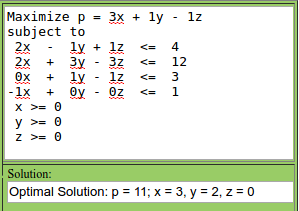
The other form that linear programs are written in is called the "slack" form (Wikipedia calls this "augmented" form, and GTech calls this the "Standard form", as if this shit isn't confusing enough.  The give away is when he starts mentioning "basic" and "non-basic" variables, which is a term used in slack form).  The main difference between the slack and standard forms is that the slack form uses equalities instead of inequalities.  It does this by introducing another variable to represent the "slack" in a given constraint.  Our example above could be rewritten in slack form thus:


Maximize   3x + 1y - 1z
subject to
 2x  -  1y + 1z + h   = 4
 2x  +  3y - 3z + i   = 12
 0x  +  1y - 1z + j   = 3
-1x  +  0y - 0z + k   = 1
 x, y, z, h, i, j, k >= 0

Unfortunately this breaks the solver I was already using, so I had to find another one.  The solver on Wolfram Alpha wasn't flexible enough either, but PHPSimplex got the job done with some massaging.  Notice that we get the same optimal result (x = 3, y = 2, here represented as X1 and X2), but we also get the "slack" in the third and fourth constraints.  We can confirm easily enough... -x <= 1  has slack 4 (i.e. 1 - (-3)), and  y <= 3  has slack 1 (i.e. 3 - 2).  This is one instance where the book really fell short for me.  While the explanation of the conversion of standard form to slack form wasn't incorrect in CLRS, it wasn't exactly helpful.  Ironically, it was Wikipedia that actually helped me get it in a form that I could feed to a solver.  Go figure...

Duality

The way Roughgarden introduces the idea of duality is through an exercise of trying to find a tight upper bound for an example linear program.  This problem of finding an upper bound on the optimal objective value for the original, or primal, linear program can itself be represented as a linear program.  Big Papa (CS170) probably has the most memorable example illustrating duality in lecture 19 of the Berkeley course, mostly just because he is such a character.

One way to define a dual linear program is using the matrix and vector format described above for the Standard Form.  Basically we take a transpose of the whole problem, so the primal that looks like this:

maximize c'x

subject to Ax ≤ b

and x ≥ 0

becomes a dual that looks like this:

minimize b'y
subject to A'y ≥ c
and y ≥ 0

Continuing with the same simple LP from earlier, I can flip everything around and end up with the following LP (for whatever reason PHPSimplex gave me an incorrect solution to this, so I went back to the zweigmedia site):

Notice that the optimal solution value of 11 is the same as the optimal value for the primal.  This is no coincidence.  Like max flow and min cut in network flows, LPs and their duals have a complementary relationship.  Weak duality basically says that any feasible solution in the primal is ≤ any feasible solution in the duel, and Strong duality says that the optimal solution to the primal is equal to the optimal solution to the dual.

The infeasibility and boundedness of the primal and its dual is an inverse relationship.  That is, if a primal is infeasible, its dual is unbounded, and vice versa.

Algorithms for solving LPs

The Simplex algorithm is given the most air time, and is the only algorithms actually covered by most of the classes.  For the most part, the ellipsoid and interior point methods are acknowledged, but they aren't really explained (except, of course, by Roughgarded, but even he spends most of his time on Simplex IIRC).  The ellipsoid method was created in 1979 by Khachiyan, and though it exhibits polynomial worst case performance, it apparently is pretty slow in practice.  The interior point method by Karmarkar in 1984 is fast in both theory and practice.  Although Simplex is exponential in the worst case, it is fast in practice.

Of all the lectures covering Simplex, I think the one that did the best job bringing it home for me was the MIT lecture.  I could have been the fact that I watched it last, but even going back and watching the GTech lectures again, I get lost.  I think Srini just does a better job explaining it.  Papa also does a step by step example starting around minute 20 in CS170 lecture 21 that is excellent.

The starting point for Simplex is a feasible basic solution.  A simple example of this might be the origin (when the origin is a feasible solution).  A basic solution is represented in slack form, so the origin has all the decision variables set to zero, and all the slack variables will be "full slack".  The algorithm doesn't require you to start at the origin by any means... any feasible solution will do.

Initially, the variables in the objective function are the "non-basic" variables, and the slack variables are the "basic" variables.  In this context, "basic" is related to basis, as in the basic variables make up the basis of the solution.  Or something like that.  It isn't basic as in "simple" or "fundamental".

The algorithm proceeds something like this:

• if you have a non-basic variable with a positive coefficient, swap it into the basis. This variable is often written as Xe  (i.e. "X sub e"), and is called the entering variable.
• a basic variable needs to be "swapped out".  This is going to be the variable corresponding to the most restricted constraint.  This is called the leaving variable and is written Xl (X sub el).
• to accomplish the swap, rewrite the constraints with the entering variable and the leaving variable in switched roles (either as a slack variable or as a constraint variable)
• Set non-basic variable to zero and tada the object value has not decreased in value and has probably increased.

Without working an example, Simplex is hard to explain.  The best thing I can suggest is to watch Srini work the example problem (starts at the one hour mark pretty much on the dot).

Other interesting LP stuff

Tim Roughgarden and Papa both cover max flow, minimax, and multiplicative weights.  Papa uses the "Penalty Kick Game" to demonstrate the Minimax theorem, whereas Tim uses a rock-paper-scissors example.  Tim's coverage felt less hand-wavey. probably owing to the fact that his background is in game theory.  I'd seen minimax before as part of CS188, this was more of a theoretical take on it.

Multiplicative weights is an online algorithm for minimizing "regret" in an ongoing game.  So think of the rock paper scissors example.  With perfect hindsight, we can determine what we could have gotten had we played the same move every time.  The difference between this "best oracle" score and the score we got is called "regret".  Our strategy can't be deterministic, because an adversary can construct a pathological input that will do terrible, but we want to do better than a uniform random guess.  So we "learn" as we go, giving winning moves gradually more weight and losing moves less weight.  By doing this we can reduce regret to an arbitrarily small number by repeating the game.  These sections were heavy with the game theory and math, and I can't do it justice in a paragraph.

Max flow can be formulated as a linear program, with CS170 and CS261 both spending a good deal of time doing examples and proofs.  It's basically a mechanical process of creating constraints corresponding to edge capacities, constraints enforcing flow conservation, and non-negativity constraints.  One interesting side effect of this form of the flow problem is that adding edge weights is basically a trivial matter, whereas with the standard combinatorial algorithms it created quite a mess.  Unfortunately when they got real deep in the weeds with the math my eyes kind of glazed over and I got less out of it.  But hey, I tried haha.

Week 10: Complexity

MIT Lectures 16-18, Recitations 8 & 9
Stanford CS261 Lectures 15-20.
GTech units on P vs NP, NP Completeness, NPC Problems, Approximation.
Berkeley CS170 (2012) Lectures 22-25.
Rob Conery - How Complexity Theory Can Save Your Job
Steven Skiena - The Algorithm Design Manual

P vs NP

The Georgia Tech material touches on some of the "theory of computation" type terminology we see in the book.  A "problem" is formulated as a "language"... or some such business.  The book put me to sleep.  I think the lectures, particularly the MIT lectures, did a much better job of conveying the material.  And while I got the sense that perhaps Rob Conery was maybe abusing some notation (and I question his complexity analysis on his "co-occurance" query), it was nice to kind of get that "real world" angle on an otherwise very academic topic.

So here are the basics:

• P is the class of problems that are solvable in polynomial time.
• NP is the class of decision problems that are verifiable in polynomial time.
• NP-complete are those problems that are in NP, and are at least as hard as everything else in NP.
• NP-hard problems are at least as hard as those in NP, and may not even be in NP at all.  They may not even be computable.  The halting problem and the min-cost optimization TSP are examples of problems not in NP that are NP-hard.
• There is a crap ton of other complexity classes out there, but that is for another course.

Papa put a lot of emphasis on the fact that NP deals with decision problems.  So to be NP-complete, a problem first had to be a decision problem.  A decision problem is a problem with a boolean result.  Many optimization problems, like the Traveling Salesman Problem (TSP), can be restated as decision problems.  So instead of trying to find the minimum cost route that visits all nodes once (classic TSP), we might ask if a route exists with cost less than k.

It is commonly believed (but as yet unproven) that P is a strict subset of NP.  Meaning there are decision problems for which polynomial time algorithms are not believed to exist.  This is the "P = NP" or "P ≠ NP" problem.

NP-complete problems and reductions

Many of the lectures devote a great deal of time to characterizing NP-complete problems.  The various flavors of satisfiability (SAT) are pretty common, particularly 3-SAT (or 3-CNF-SAT if you are picky about abusing nomenclature).  I thought Papa got kind of hand wavey regarding the close relationship of cliche, vertex cover, and independent set.  But they are practically the same problem once you understand the relationships:

A maximum clique is a maximum independent set in the complement graph (i.e. ever edge in G is not in G', and every edge not in G is in G'), and the minimum vertex cover is the complement of the max independent set, so {VC} ∪ {INDSET} = {V}.

Other problems don't convert quite so neatly, but it is still possible to express any NP-complete problem as any other problem (by definition).  This process of reformulating a problem to solve another is called a reduction, and it is covered ad nauseum.  The most important point to remember when doing a reduction is the direction.  If I am trying to prove that Mario Brothers is NP-complete, then I need to express another NP-complete problem as an instance of Mario Brothers.  Demaine demonstrates this with a number of Mario Bros "gadgets" that essentially simulate 3-Sat by creating a level in the game.  If we had a polytime solver for the game, we could use it so solve 3-Sat and prove that P=NP.  But since 3-Sat can be expressed using Mario Bros, that means Mario is NP-complete.  It was definitely the most interesting take on an NP-completeness reduction I've seen, and makes me think that 6.890 might be worth a closer look.

Both Papa and Demaine work a reduction of 3D Matching from 3-Sat.  Demaine explains very well the use of the "wheel" gadget, the clause gadget, and the "garbage collection" as he called it.  Papa, honestly, doesn't explain it nearly as clearly.  If I hadn't already seen Eric explain it, I probably would have been pretty confused.  Though the way he uses "girls boys and pets" as a vehicle is pretty funny.  So it's worth watching for that aspect at least. =P

One important takeaway from Roughgarden's class was that just because a problem is NP-complete or even NP-hard, it doesn't mean we have to settle for brute force algorithms.  In lecture 19, he gives examples of algorithms for vertex cover, 3-Sat, and TSP that were much better than brute force.  Vertex cover is solved with a kernelization approach, that basically reduces the problem down to a much smaller instance and then solves with brute force (kernel approach also covered in MIT lectures).  TSP can be solved using DP, which reduces complexity from n! to n² * 2^n.  3-Sat can be solved with a randomized algorithm (Schoening's Algorithm) that succeeds with high probability after running for some exponential amount of time (but not a terrible exponential, something like 4/3 raised to the n times some roots and logs).

Approximation Algorithms

If we need a polynomial time algorithm for a problem, and can tolerate a result that is less than optimal, there are a number of hard problems that admit fast approximation algorithms.  Approximation algorithms have their own set of vocabulary:

• PTAS - Polynomial Time Approximation Scheme.  Approximations can be made arbitrarily accurate by trading off time.  Takes a parameter ε, and results in a solution that is within 1 + ε of optimal. Complexity must be polynomial in n, but may be exponential in ε
• EPTAS - Efficient Polynomial Time Approximation Scheme.  Exponent on n is constant independent of ε
• FPTAS - Fully Polynomial Time Approximation Scheme.  Algorithm must be polynomial in both n and ε 
• FPT - Fixed Parameter Tractable.  Problems that can be solved in time polynomial in the input size (but still exponential in another function).  (Lecture 19 of CS261, Demaine covers in MIT Lecture 18)

Approximation algorithms for Metric Traveling Salesman (that is, TSP that obeys the triangle inequality) are covered by several of the classes.  The 2-approximation algorithm (that is, it always produces a tour at worst 2x optimum) constructs a minimum spanning tree over the vertices, doubles the edges to form a Eulerian tour, then uses "shortcuts" to shorten the tour by skipping over vertices that have been visited already.  Because the graph obeys the triangle inequality, these shortcuts are guaranteed to not lengthen the tour (though they won't necessarily shorten it either, think of a graph where all the vertices are in a line).  Because the MST is ≤ OPT, and the approximation is ≤ 2 x MST (because of the Eulerian tour), the approximation is guaranteed to be ≤ 2 x OPT.

Another algorithm, Christofides algorithm, does even better, being no worse than 3/2 x OPT.  Roughgarden covers these in lecture 16.  There was actually an article in wired about an "improvement" to Christofides algorithm that makes it about one one-billion-trillion-th of a percent better (or some other such stupid small fraction).

Roughgarden covers the greedy approximation algorithm for set cover in some depth in lecture 17 (not to be confused with set coverage, which is a related problem he covers in lecture 15).    I think both of these were not constant factor approximations, but instead something kind of log-ish in the input size.  The greedy algorithm works by selecting the set with the most uncovered nodes.

One approximation algorithm I found very interesting is the randomized algorithm for vertex cover.  This algorithm works by selecting random edges from the graph, and adding both endpoints to the cover.  This stupid simple algorithm results in a 2-approximation of the optimum set cover.  Contrast with a "smarter" algorithm that selects nodes with the highest degree to add to the cover, which results in a log(n) approximation.  Papadimitriou covers this same random approximation algorithm in lecture 25 of CS170 (2012).

He also covers linear programming relaxation in lecture 17, and a semi-definite programming relaxation in lecture 20.  The relaxation techniques were very cool but I'd be lying if I said I understood more than 10% of them. Lecture 18 covers randomized algorithm analysis, though Roughgarden goes much deeper into the weeds (Markov, Chernoff, "linearity of expectations", etc.), and again mostly lost me.

Knapsack admits a FPTAS that basically works by truncating the small order bits on large instances and running the classic DP solution.  Knapsack is a funny problem in that it's a pretty common example for DP, and it seems to run efficiently, but it's pseudo-polynomial, meaning it's complexity is tied to the value, rather than the size of the input.  Because the value of the input has an exponential relationship with the size of the input, it is actually an exponential problem.  The approximation algorithm will allow you to trade time for accuracy (meaning you can get as close as you want... 10%, 1%, 0.1% of optimum, whatever).  Just lop off fewer low order bits.  Papa covers this algorithm (lecture 23), and Roughgarden does as well (lecture 15).

Week 11: Distributed Algorithms

MIT lectures 19 & 20, Recitation 10

The last few weeks should be a breeze compared to the last few weeks of material. No more quadruple coverage, as the last bits are unique to MIT.  Nancy Lynch covered a few distributed algorithms for spanning trees and leader election in graphs.  She used slides instead of the chalkboard, which I didn't like as well (particularly in lecture 20 since the video was way out of synch with which slide she was on).

The first big idea for distributed algorithms is symmetry breaking.  Basically, if you have a bunch of identical nodes, trying to run identical distributed algorithms, then there is no way to make progress.  The simple solution is to introduce UIDs for the nodes, which gives these algos a basis of comparison with which to make decisions.

The other big idea was synchronous vs asynchronous algorithms.  Synchronous algorithms basically worked in "rounds", where every node took one "step" all at the same time.  This allowed the algos to retain a certain degree of determinism.  With asynch algorithms, that determinism goes out the window.  The shortest paths tree algorithm highlighted this distinctions quite well.  In the synchronous version, you could count on the nodes sending messages in a rational order, and a node could chose it's parent pretty easily.  With the asynch version, nodes had to keep correcting their parent pointers and weights as new information hit them from every which way.

Complexity in these algorithms was measured a little different.  It often makes sense to discuss the number of messages generated by an algorithm, in addition to the "time" or "number of rounds".

The last big idea in this algorithms is the challenge of termination.  It's a little trickier in some of these graphs, especially if we don't know the value of n.  One strategy for this is convergecast, which is sort of the inverse of a broadcast.  Basically, a node is done when all its subtrees (non-parent neighbors really) are done, OR it has nothing to do (which is sort of like the base case).  When a node is done, it sends a "done" message to its parent.  When the root node has received done messages from all its neighbors, we know the whole algorithm is done, and the root can send a message to the whole graph if need be.

The recitation covers a leader election algorithm in a kind of "ring" graph.  The first, fairly naive algorithm generates O(n²) messages.  The more interesting algorithm (called Hirshberg-Sinclair according to the notes) has weak candidates go inactive earlier, to reduce the overall message complexity to O(n log n).  It took me a couple passes to wrap my head around it, but I think I get it:

In this example, each row represents a round, with the top row representing the first round.  At first, every node sends a message one hop in each direction.  If a node gets a message that is high than it's own value, it sends it back.  Any nodes that get both messages back survive to the next round.  At the end of the round, the inactive nodes record the max value they saw.  Roughly half the nodes are eliminated.

In the next round, each message is passed two hops.  If a node gets a message that is strictly less than their own value (or the max they've seen), then the message dies.  At the end of this round, only two nodes are still actively creating messages (87 and 94).  In round three, the messages go 4 hops.  87 does not get it's right message back (it finally overlaps with 94).  The last round is basically just 94 sending a message n/2 hops in either direction to update the whole board.

The case of a sorted list of nodes is interesting.  In the first round, every node but the max dies, then the  remaining rounds are just the max gradually propagating out its value:

In the first round, 16 produces 4 messages (2 out, 2 in), 1 produces 2 messages (2 out, 0 in), and every other node produces 3 messages (2 out, only left returned), for a total of 48 messages.  The remaining rounds are basically best case, as 16 sends 2 messages 2^i hops in either direction and gets everything back.

Week 12: Cryptography

MIT lectures 21 and 22, and recitation 11, give a very high level introduction to concepts in cryptography, related to hashing, encryption (particularly public key), and digital signatures.  I actually touched on some of this stuff for the 70-486 cert test (encryption, hashing).  Theory meets practice... =)

Cryptographic hash functions are in wide use for a variety of purposes.  It has been best practice for some time to store password hashes instead of plain text (not to mention salting and stretching, such as in PBKDF2).  Hash functions intended for these purposes have several desirable traits:

• Deterministic - the same input always produces the same hash
• One way - the original message cannot be derived from the hash value
• Collision resistant - it is not feasible to produce two different messages with the same hash
• Target collision resistant - given one message, it is infeasible to produce another with the same hash 

Two common hash functions, MD5 and SHA-1, have been successfully broken, such that is it possible to generate colliding documents.  Researchers created colliding documents for MD5 in 2005, and attackers were able to exploit this same weakness to forge certificates in 2012.  Google created PDF documents with colliding SHA-1 hashes in February of 2017 (article at shattered.io).  Source control systems such as git and svn are affected by this vulnerability as well.

To introduce the motivation behind public key encryption, Srini poses a puzzle.  Suppose we have Alice and Bob, and they live on two separate islands.  They want to send messages to each other, but the only means of transport between the islands are a band of pirates.  These pirates will open any chest that is unlocked, so how does Alice get a message to Bob?

The answer seems so simple... once you know it.  The solution is for Alice to send her message in a locked box, then Bob also locks it and sends it back to her.  She removes her lock and sends it back to Bob with only his lock.  Now he can open the box and get her message.  If Alice and Bob really trusted each other, they could exchange keys in this manner, and then for subsequent message exchanges they could open each others locks, and it would be much quicker (analogous to the way public key encryption is used to exchange secret keys so that subsequent communications can use synchronous encryption, which is much faster).

Public key encryption is an encryption scheme which uses a pair of keys - a public key and a private key.  The public key is visible to everyone, whereas the private key is kept secret.  This type of set up enables two very important applications:

• secure message passing - A message is encrypted with the recipient's public key.  The message can only be decrypted using the recipient's private key.
• digital signature - A message is encrypted with the signers private key.  Anyone can decrypt the message with the public key, certifying that the sender is the only one who could have encrypted it. 

Diffie-Hellman key exchange is arguably the earliest public key encryption protocol.  The wikipedia page does a pretty good job of illustrating the concepts involved, both in abstract (using paint colors) and mathematically (using small, understandable numbers).  In practice the numbers involved have thousands of bits and would be pretty unintelligible to mere mortals.  The takeaway is that this algorithm allows parties to establish a shared secret over an insecure channel.  Once the shared secret is established, subsequent communication can take place using symmetric encryption (as in the Pirate puzzle when Alice and Bob send each other keys). RSA is basically an implementation of Diffie-Hellman... I think.

The recitation spends some quality time with digital signatures and how they are implemented using, basically, the inverse of RSA.  The "naive" inverse of RSA is broken because of some of the mathematical properties of the keys, but hashing the message with a cryptographically secure hash and signing that fixes these issues.

While RSA uses factorization and large prime numbers, there are also public key crypto schemes that use other one way functions, with Knapsack being one covered in class.  Knapsack based public key cryptosystems have been known since around the same time as RSA was developed, but have been broken by a number of attacks.  Ling mentions that Knapsack based systems can run much faster, and seems to indicate that there may be some versions that are unbroken.  The wiki page mentions that such schemes may be more resistant to quantum computing attacks.

Message authentication code is the symmetric analog to digital signature.  MAC has only the secret key, and signs a message by concatenating the key to the message and hashing them (subject to some restrictions on how they are concatenated and which hash algorithm is used).

Ling also presents the problem of verifying file integrity on a remote server (something like Google Drive).  The problem with MAC in this scenario is that, assuming the MAC is stored with the file, Drive could just serve us up a stale previous version of the file (along with it's valid, stale MAC).  One solution is to compute a hash for every file, which we then store locally.  When we get a file, we compare its hash to the one we have, and if they match we know we have a valid file.  One drawback of this approach is that we need to store O(n) hashes.  One way around this (allegedly) is the use of the hash tree (Merkle tree), which creates a binary tree of hashes over the files (hash the files, hash the hashes together in pairs, until we get to the root hash).   Though I didn't really understand how this helped us, since it wasn't clear to me where the tree was stored (which would have more hashes than just a list of file hashes)...

Week 13: Cache-oblivious Algorithms

The last two MIT lectures (23 and 24) cover cache-oblivious algorithms.  These algorithms are covered in some depth in 6.172 (surprisingly, it isn't mentioned as a follow up course at the end of the last lecture...)

The memory hierarchy in a computer is a model for the many layers of caching that exist in a computer.  The CPU itself has a few registers where it stores data, then there are the various chip caches (L1-L3 or L4), main memory (RAM), flash memory (in some hybrid HDD's, though now SSD's are becoming more of a thing), HDD, and perhaps even the local network or internet.  As you get farther away from the CPU, the latency of these caches becomes longer and longer (Latency Numbers Every Programmer Should Know), although with clever architecture the "bandwidth", or total data throughput, can be increased almost arbitrarily.  One way to hide latency is by "blocking", or pulling back large chucks of data whenever any data is requested. By reusing the data already in a faster cache (a concept called "temporal locality"), we avoid having to call up to slower caches or datastores for the data we need.

To analyze the cache performance of our algorithms, we use the "External memory model", which is basically an abstract way of thinking about our memory accesses.  In this model, our CPU has the use of a cache made up of M words, divided into blocks of size B (so say we have a block of 64 bytes, and we have 1000 blocks, we would have a 64k cache).  While it is possible to write algorithms that take advantage of knowing M and B, these types of algorithms have their drawbacks.  For one thing, different levels of the memory hierarchy have differing values for M and B, so although a tuned algorithm may optimize for the L1 cache, it won't be optimized for anything else.

The cache-oblivious model takes the same basic construct as the external memory model, and adds the restriction that the algorithm doesn't know M or B.  In other words, our algorithm has to work for ALL values of M and B.  What this means is that the algorithm is more portable, and also that it works well for every level of the memory hierarchy.

The general theme I got from these two lectures is that we want our data to be physically close together in memory (spacial locality).  The first time a value is read, instead of just grabbing the one value, we grab a "block" of data, caching the neighbors of the data we were interested in.  This means that if subsequent reads use data that is nearby, these reads are essentially "free" because we've already loaded the block.  It's only when we cross block boundaries that we really pay for memory accesses.  I made a few graphics to illustrate this relationship:

I did a quickie "simulation" in a spreadsheet comparing a bunch of random reads with a series of sequential reads.  This is kind of worst case vs best case.  The idea is that each cache is one block, so changing blocks at any level reloads the cache.  The random reads rarely get to take advantage of cached data (never at the lowest level).  Granted it's a contrived example, but still interesting:

Demaine covers several cache-oblivious divide and conquer algorithms, including "scans" (basically anything that just reads though an array), median finding, matrix multiplication, search, and sort.  Particularly interesting was the way the search algorithm worked.  First we pre-process the data by sorting it.  We can then overlay a full binary tree over the data, which in the naive sense gives us O(log n) lookup but is not cache efficient.  What we want to do is add nodes to the tree in such a way that the top sqrt N nodes are in a continuous array.  Then as we traverse the tree, we are minimizing the number of cache boundaries we have to cross.  This layout is called the "van Emde Boas" layout because it resembled a vEB tree structure.

There are a couple of strategies for evicting cache values when we need to free up space for new data.  On is to evict the oldest block (FIFO), another is to evict the least recently used block (LRU), and another is to evict a random block.  Demaine contends the first two are decent strategies, and the random eviction strategy is probably also good in expectation.

Eric and Srini cap it off with a frisbee throwing contest in the spirit of William Tell.  I love these guys lol.

Bonus: Online Algorithms (Stanford)

Introduced in CS261 lecture 11 (Multiplicative Weights), and does into depth in lectures 13 and 14.

Min makespan scheduling is the first online algorithm problem Roughgarden analyzes.  This problem says we have m machines, and a stream of jobs with weights (processing time basically), and we want to minimize the "makespan", which is basically the maximum load on all our machines.  So if we have two machines with load 5 and 3, our makespan is 5.  A good solution for this problem is to assign incoming jobs to the machine with lowest current load.  This algorithm is at worst 2x OPT (the best we could have done in hindsight).  Another way to say this is that the algorithm is "two competitive".

Steiner tree problem is a graph problem.  We have a weighted undirected graph to start (offline), and arriving online are vertices of the graph.  The problem is that we need to maintain connectivity between all the terminals.  Because all the edge weights are non-negative, we end up with spanning trees.  The greedy algorithm simply connects the incoming terminal to the existing terminal with the cheapest edge (the graph is complete, so there is always a one-hop edge connecting a new terminal to the existing graph).  This algorithm isn't constant factor competitive, instead being Ω(lg k) competitive where k is the number of terminals.  Incidentally, this is the best that can be done for online Steiner trees.  The proof uses the same trick we saw in the Metric TSP 2-approximation.

Online bipartite matching - We have vertices divided into L and R, we have all of L up front, and the vertices in R show up online, along with all their incident edges.  We have to connect the vertex when it shows up (if we can) and this matching is permanent.  The goal is a max cardinality matching.  One real world application is web advertising (L is advertisers, R is consumers).  There is no deterministic algorithm with a competitive ratio better than 0.5, but randomized algorithms can do a bit better.  Tim goes pretty deep on the proofs with the LP duality and whatnot... and I'm just done.