My CS188 Post (Berkeley AI class)
My Github Repo for this class
A first look at basic discrete probability, how to interpret it, what probability spaces and random variables are, and how to code these up and do basic simulations and visualizations.
Modeling uncertainty requires two "ingredients":
My Github Repo for this class
Week 1: Introduction to probability and computation
Modeling uncertainty requires two "ingredients":
- Set of all possible outcomes, i.e. the "sample space" denoted as omega Ω
- Probability of each outcome, denoted as P with two vertical lines (but I'll just use uppercase P)
In general, P(S) means "the probability that S happens"
In Python:
model = {'heads': 1/2, 'tails': 1/2}
sample_space = set(model.keys)
Sample space is collectively exhaustive, and an experiment results in exactly one outcome (not zero, not two...). Probabilities are in range [0, 1], and all probabilities in model must sum to 1. In this class, sample space is always finite.
An "event" is the occurrence of some subset of possible outcomes from the sample space. In a model of two coin flips with Ω = {HH, HT, TH, TT}, examples of events might be "2nd coin is T" or "at least one flip is H". These two events can be represented as subsets o the sample space, i.e. {HT, TT} and {HH, HT, TH} respectively. An outcome can trigger more than one event, for example HT would trigger both of the above events.
The probability of an event is the sum of all the outcomes in the set for that event.
Because an event is a set (actually a subset of Ω), we can talk about the union, intersection, and complement of an event, as with any set. Two special events are Ω (full set) with a probability of 1, and ϕ (empty set) with probability of 0.
Random variables:
In general, a random variable is a function that maps from the sample space onto an "alphabet" of outcomes. Essentially relabels the outcomes. The probabilities of the new labels can be represented in a probability table, and may also be called a probability mass function (PMF) or a probability distribution.
Incorporating observations using jointly distributed random variables and using events. Three classic probability puzzles are presented to help elucidate how to interpret probability: Simpson's paradox, Monty Hall, boy or girl paradox.
The relationship between two random variables can be represented as a joint probability table (also called a joint probability distribution). So if we have variables W and T, the joint distribution is written as P(W, T) with a comma between the variables. We can calculate the distribution for either random variable from this joint distribution through a process called marginalization ("summing out").

For more than two random variables, the process is essentially the same, the summation process is simply repeated for each variable we want marginalized:

A conditional probability distribution sets one random value to a fixed value and renormalizes. This is denoted with a pipe | in the probability, with the "known" values on the right of the pipe. P(A | b1) is read as "probability distribution of A given B is b1", which would give us {a1: 0.9, a2: 0.1, a3: 0.0}. (See Week 7 of the AI post).

We can think about this more generally by looking at event B rather than just the singular event ω. Now, if A occurs, and we want to know the probability that B occurs, we have to look at the intersection of A and B (the probability of all other B occurring is 0). Therefore:
P(B | A) = P(A∩B) / P(A) //Conditional probability of B given A
This can also be written as
P(A∩B) = P(A) * P(B | A) //Product rule
We know from above that P(A | B) = P(A∩B) / P(B), which we can rearrange as P(A∩B) = P(B) * P(A | B). What is interesting is that this gives us a different definition of P(A∩B), which we can plug into the formula we had for P(B | A) to give us:
P(B | A) = P(B) * P(A | B) / P(A)
This is Bayes Rule. It is useful because it allows us to compute a conditional probability when we have the inverted conditional (which is often the case in inference problems...)
We can partition a sample space. If we have B1...Bn, where all Bx are disjoint, and all Bx sum to the sample space Ω, then we can reformulate P(A) as P(A∩B1) + P(A∩B2) + ... + P(A∩Bn)
The product rule and inference with Bayes' theorem. Independence: A structure in distributions. Measures of randomness: entropy and information divergence. Mutual information.
Product rule for events:
P(A∩B) = P(B) * P(A | B)
The product rule for random variables is similar:
P(A, B) = P(A) * P(B | A) = P(B) * P(A | B)
This means that if we have P(A) and P(B | A), we can calculate the full joint distribution P(A, B)... did this a lot in the AI class. For multiple random variables, we can keep introducing them to the right hand side, conditioned on everything that has been introduced already (wow, that makes so much sense </sarcasm>).
It looks like this:
P(x1, x2, x3, ... xn) = P(x1) * P(x2 | x1) * P(x3 | x1, x2) * ... * P(xn | x1 ... xn-1)
Each of these expressions on the right hand side is called a factor.
Independence was a topic also heavily covered in the AI class. There are a couple types of independence: Mutual (Marginal) Independence, and Pairwise (Conditional) Independence
If two events are independent, then P(A∩B) = P(B) * P(A)
This also implies that P(B | A) *P(A) = P(B) * P(A) which, after canceling P(A) from both sides, leaves us with P(B | A) = P(B). In other words, knowing the value of A gives us no information about B.
This can also be written with the joint distribution format:
P(A, B) = P(A) * P(B)
We say that A is independent of B (or vise versa), which can be written as A ⊥ B (though it should properly be a "double up tack" ⫫, it doesn't look quite right in my standard font... doh!).
Multiple variables are said to be "mutually independent" is knowing any of them tells us nothing about the rest. P(x,y,z) = P(x) * P(y) * P(z)
Pairwise independence is a weaker form of independence in which knowing any one variable doesn't tell us anything about the others, but knowing more than one may break independence. So
P(x,y) = P(x) * P(y) AND
P(x,z) = P(x) * P(z) AND
P(z,y) = P(z) * P(y)
but
P(x,y,z) ≠ P(x) * P(y) * P(z)
This can also be described as two variables being independent given the third variable. So
P(x, y | z) = P(x | z) * P(y | z)
Marginal Independence and Conditional Independence do not imply each other. Variables can be one without being the other. (There are several videos walking through each, which closes mirror what was done in the AI class regarding conditional independence and graph shapes)
Expected values of random variables. Classic puzzle: the two envelope problem. Probability spaces and random variables that take on a countably infinite number of values and inference with these random variables.
The expected value of a random variable can be thought of as the average value of a lottery. If we have a lottery that you pay $1 to play, and have a 1 in 1,000 change of winning $1000, the expected value is -$1 + $1,000 * (1/1000) or 0.
In general, the expected value of a discrete random variable (where the labels are numbers) is the sum of the labels times their associated probabilities. Essentially a weighted average.
The exercises for the first section of week 4 look at variance. The first few aren't bad but then they went all cra-cra with linearity of expectation and I got in a bit over my head. I suppose it is an MIT class so I should have expected the problems to get harder and more math-heavy... yikes!
Shannon information content/self-information:
This is basically the number of bits that must be stored to represent an outcome. I remember encountering this in the AI course (after some digging I found it: 22.5 minutes into Lecture 23 of the Berkeley course; Patrick Winston covers the related concept of entropy in Lecture 11 of the MIT AI course... anyway...).
Generally, the self-information for an event A is defined as log2(1 / P(A))
For a deterministic outcome, self-information is 0 bits
For a fair coin, self information is 1 bit (log2( 1 / .5) == log2( 2 ) == 1)
As P(A) increases, the number of bits to describe the event decreases.
Shannon entropy:
The basic intuition is that a variable that is more random is less predictable, and therefore less compressible (requires more bits to store).
To calculate the entropy of a distribution, we first look at the Shannon information for a single outcome. For example, a fair coin with has distribution {H: 0.5, T: 0.5}. If we do n random samples, the entropy is the sum for all x in our "alphabet" of n * P(x) * log2 (1 / P(x)) [i.e. Shannon Information]. If you factor out the n, you get the average entropy of random variable X, which is denoted as H(X) or H(P(X)).
For the coin toss example, H(X) looks like 0.5 * log2( 1 / 0.5) + 0.5 * log2( 1 / 0.5) == 1 bit.
Information Divergence (Kullback - Leibler):
This gives us a way to measure of how different two distributions are based on entropy. For two distributions p and q, we calculate the entropy of p as we normally would, and then we calculate the entropy again, except in the Shannon Information portion of the formula we substitute distribution q. We then subtract the entropy of p from that of q:

which we can rewrite as:

D(p||q) = 0 iff p ≡ q , that is ∀x p(x) = q(x)
In general, D(p||q) ≠ D(q||p) (Gibbs Inequality)
Geometric Distribution
Biased coin P(H) = p
We're going to toss the coin until we get heads:
Ω = {H, TH, TTH, TTTH, ...}
P(H) = p
P(TH) = (1-p) * p
P(TTH) = (1-p)² * p
P(TTTH) = (1-p)³ * p
and so on...
Let random variable x = # of tosses until first heads appears
alphabet X = {1, 2, 3, 4...}
P(X=x) = P(x-1 tails followed by heads) = (1-p)^(x-1) * p
This is the probability mass function of random variable x
Geometric distribution consequence of geometric decay of probability as x is increased.
At this point I am really starting to feel like I got in over my head, and if it doesn't start to click soon I may give up the ghost on getting a good grade... yikes!
Some resources that were helpful on the exercises:
Computation of Kullback-Leibler (KL) using numpy, scipy docs for entropy
An "event" is the occurrence of some subset of possible outcomes from the sample space. In a model of two coin flips with Ω = {HH, HT, TH, TT}, examples of events might be "2nd coin is T" or "at least one flip is H". These two events can be represented as subsets o the sample space, i.e. {HT, TT} and {HH, HT, TH} respectively. An outcome can trigger more than one event, for example HT would trigger both of the above events.
The probability of an event is the sum of all the outcomes in the set for that event.
Because an event is a set (actually a subset of Ω), we can talk about the union, intersection, and complement of an event, as with any set. Two special events are Ω (full set) with a probability of 1, and ϕ (empty set) with probability of 0.
Random variables:
In general, a random variable is a function that maps from the sample space onto an "alphabet" of outcomes. Essentially relabels the outcomes. The probabilities of the new labels can be represented in a probability table, and may also be called a probability mass function (PMF) or a probability distribution.
Week 2: Incorporating observations
The relationship between two random variables can be represented as a joint probability table (also called a joint probability distribution). So if we have variables W and T, the joint distribution is written as P(W, T) with a comma between the variables. We can calculate the distribution for either random variable from this joint distribution through a process called marginalization ("summing out").

For more than two random variables, the process is essentially the same, the summation process is simply repeated for each variable we want marginalized:

A conditional probability distribution sets one random value to a fixed value and renormalizes. This is denoted with a pipe | in the probability, with the "known" values on the right of the pipe. P(A | b1) is read as "probability distribution of A given B is b1", which would give us {a1: 0.9, a2: 0.1, a3: 0.0}. (See Week 7 of the AI post).
We can think about this more generally by looking at event B rather than just the singular event ω. Now, if A occurs, and we want to know the probability that B occurs, we have to look at the intersection of A and B (the probability of all other B occurring is 0). Therefore:
P(B | A) = P(A∩B) / P(A) //Conditional probability of B given A
This can also be written as
P(A∩B) = P(A) * P(B | A) //Product rule
Bayes Rule (or Theorem... or Law...)
We know from above that P(A | B) = P(A∩B) / P(B), which we can rearrange as P(A∩B) = P(B) * P(A | B). What is interesting is that this gives us a different definition of P(A∩B), which we can plug into the formula we had for P(B | A) to give us:
P(B | A) = P(B) * P(A | B) / P(A)
This is Bayes Rule. It is useful because it allows us to compute a conditional probability when we have the inverted conditional (which is often the case in inference problems...)
Law of Total Probability
We can partition a sample space. If we have B1...Bn, where all Bx are disjoint, and all Bx sum to the sample space Ω, then we can reformulate P(A) as P(A∩B1) + P(A∩B2) + ... + P(A∩Bn)
Week 3: Introduction to inference, structure in distributions, and information measures
Product rule for events:
P(A∩B) = P(B) * P(A | B)
The product rule for random variables is similar:
P(A, B) = P(A) * P(B | A) = P(B) * P(A | B)
This means that if we have P(A) and P(B | A), we can calculate the full joint distribution P(A, B)... did this a lot in the AI class. For multiple random variables, we can keep introducing them to the right hand side, conditioned on everything that has been introduced already (wow, that makes so much sense </sarcasm>).
It looks like this:
P(x1, x2, x3, ... xn) = P(x1) * P(x2 | x1) * P(x3 | x1, x2) * ... * P(xn | x1 ... xn-1)
Each of these expressions on the right hand side is called a factor.
Independence
Independence was a topic also heavily covered in the AI class. There are a couple types of independence: Mutual (Marginal) Independence, and Pairwise (Conditional) Independence
If two events are independent, then P(A∩B) = P(B) * P(A)
This also implies that P(B | A) *
This can also be written with the joint distribution format:
P(A, B) = P(A) * P(B)
We say that A is independent of B (or vise versa), which can be written as A ⊥ B (though it should properly be a "double up tack" ⫫, it doesn't look quite right in my standard font... doh!).
Multiple variables are said to be "mutually independent" is knowing any of them tells us nothing about the rest. P(x,y,z) = P(x) * P(y) * P(z)
Pairwise independence is a weaker form of independence in which knowing any one variable doesn't tell us anything about the others, but knowing more than one may break independence. So
P(x,y) = P(x) * P(y) AND
P(x,z) = P(x) * P(z) AND
P(z,y) = P(z) * P(y)
but
P(x,y,z) ≠ P(x) * P(y) * P(z)
This can also be described as two variables being independent given the third variable. So
P(x, y | z) = P(x | z) * P(y | z)
Marginal Independence and Conditional Independence do not imply each other. Variables can be one without being the other. (There are several videos walking through each, which closes mirror what was done in the AI class regarding conditional independence and graph shapes)
Week 4: Expectations, and driving to infinity in modeling uncertainty
The expected value of a random variable can be thought of as the average value of a lottery. If we have a lottery that you pay $1 to play, and have a 1 in 1,000 change of winning $1000, the expected value is -$1 + $1,000 * (1/1000) or 0.
In general, the expected value of a discrete random variable (where the labels are numbers) is the sum of the labels times their associated probabilities. Essentially a weighted average.
The exercises for the first section of week 4 look at variance. The first few aren't bad but then they went all cra-cra with linearity of expectation and I got in a bit over my head. I suppose it is an MIT class so I should have expected the problems to get harder and more math-heavy... yikes!
Shannon information content/self-information:
This is basically the number of bits that must be stored to represent an outcome. I remember encountering this in the AI course (after some digging I found it: 22.5 minutes into Lecture 23 of the Berkeley course; Patrick Winston covers the related concept of entropy in Lecture 11 of the MIT AI course... anyway...).
Generally, the self-information for an event A is defined as log2(1 / P(A))
For a deterministic outcome, self-information is 0 bits
For a fair coin, self information is 1 bit (log2( 1 / .5) == log2( 2 ) == 1)
As P(A) increases, the number of bits to describe the event decreases.
Shannon entropy:
The basic intuition is that a variable that is more random is less predictable, and therefore less compressible (requires more bits to store).
To calculate the entropy of a distribution, we first look at the Shannon information for a single outcome. For example, a fair coin with has distribution {H: 0.5, T: 0.5}. If we do n random samples, the entropy is the sum for all x in our "alphabet" of n * P(x) * log2 (1 / P(x)) [i.e. Shannon Information]. If you factor out the n, you get the average entropy of random variable X, which is denoted as H(X) or H(P(X)).
For the coin toss example, H(X) looks like 0.5 * log2( 1 / 0.5) + 0.5 * log2( 1 / 0.5) == 1 bit.
Information Divergence (Kullback - Leibler):
This gives us a way to measure of how different two distributions are based on entropy. For two distributions p and q, we calculate the entropy of p as we normally would, and then we calculate the entropy again, except in the Shannon Information portion of the formula we substitute distribution q. We then subtract the entropy of p from that of q:

which we can rewrite as:

D(p||q) = 0 iff p ≡ q , that is ∀x p(x) = q(x)
In general, D(p||q) ≠ D(q||p) (Gibbs Inequality)
Geometric Distribution
Biased coin P(H) = p
We're going to toss the coin until we get heads:
Ω = {H, TH, TTH, TTTH, ...}
P(H) = p
P(TH) = (1-p) * p
P(TTH) = (1-p)² * p
P(TTTH) = (1-p)³ * p
and so on...
Let random variable x = # of tosses until first heads appears
alphabet X = {1, 2, 3, 4...}
P(X=x) = P(x-1 tails followed by heads) = (1-p)^(x-1) * p
This is the probability mass function of random variable x
Geometric distribution consequence of geometric decay of probability as x is increased.
At this point I am really starting to feel like I got in over my head, and if it doesn't start to click soon I may give up the ghost on getting a good grade... yikes!
Some resources that were helpful on the exercises:
Computation of Kullback-Leibler (KL) using numpy, scipy docs for entropy
How many times to roll a dice
When I first started approaching this assignment, I felt like I was in waaaaay over my head. But taking it a step at a time (and leaning on Google Sheets) helped me slog through it.
Part (b)
This part comes down to implementing the following formula:

PX(x) is given as {0: 0.6, 1: 0.4}
PY|X(yn | x) is {x=0: {0: 0.7, 1: 0.3}, x=1: {0: 0.98, 1: 0.02}
and observations y = [0, 0, 1]
So, to compute the posterior probability P(X | Y), for x=0 and x=1, first we calculate the unnormalized product:
x = 0: 0.6 [PX(x=1)] * 0.7 [PY|X(y[0] | x=0) * 0.7 [PY|X(y[1] | x=0) * 0.3 [PY|X(y[2] | x=0)
x = 0: 0.0882
x = 1: 0.4 [PX(x=1)] * 0.02 [PY|X(y[0] | x=1) * 0.02 [PY|X(y[1] | x=1) * 0.98 [PY|X(y[2] | x=1)
x = 1: 0.0076832
When we normalize, we get the posterior probability {0: 0.91987, 1: 0.08013}
Part (c)
This part has us creating the likelihood distribution P(Y|X). The distribution is determined by the following formula, where x and y can take values from some range of numbers from 0 to M-1 (so if M=4, then the domain is [0,1,2,3]):

Now at first this really tripped me up (and plenty of other folks, based on the discussion forums...). I found it helpful to build out an example in Google Sheets.
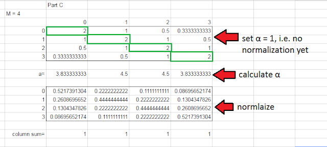
The intuition here is that the columns represent the probability of a true rating x given a user rating y. So if the user rated it a 0, there is a 52% chance that the true rating is 0, 26% chance it is 1, 13% chance it's 2, and a 9% chance it's 3. Once I wrapped my head around that, the rest got a lot easier. And really this was the last of the hard coding.
Parts (d - g)
The rest was pretty straight forward. Part (d) really just involves looping over the movies and passing a calling the code we wrote in part (b) to compute posterior probabilities (using the code from part (c) to calculate the likelihood distribution).
Part (f) is calculating the entropy for a distribution... which I just delegated to the scipy method and thus didn't have to dick around with accounting for 0log(0) and all that. Work smarter not harder...
And then part (g), which is plotting the average entropy for all the movies based on how many ratings we use to calculate the model. I first pass was jacked up because of a stupid bug in my code for computing all the posterior entropy numbers. Once I sorted that, however... it was smooth sailing. Now if they'd just post the grader...
Introduction to undirected graphical models as a data structure for representing probability distributions and the benefits/drawbacks of these graphical models. Incorporating observations with graphical models.
This weeks material is pretty light on the lecture content. Some review of Big O notation. One of the big take aways is that storing a complete joint probability table for n random variables, each of which can take k different values, requires k^n space to store. So for problems with many random variables, a more efficient mechanism is required. Enter graphical models.
In a graphical model, our probability space is represented by a collection of nodes and edges. Each individual node has a probability associated with it, what is referred to as a potential function. There is usually more than one way a given graphical model can be represented. Take the simple example of two knows connected with one edge:
(x1)----(x2)
We can represent the joint probability using the phi symbol: ψ12 = P(x1, x2)
We can also break the joint probability down using the product rule: P(x1, x2) = P(x1) * P(x2 | x1)
... which we can notate using phi for the singleton probability: φ1 = P(x1), ψ12 = P(x2 | x1)
... note that this ψ12 is different from the ψ12 defined above, but the notation convention makes them confusing.
Finally, we can use the product rule the other way: P(x1, x2) = P(x2) * P(x1 | x2)
... which we can notate as: φ1 = P(x2), ψ12 = P(x1 | x2)
When we can make assumptions regarding conditional independence, it starts to define the structure of the graphical model. Take the following graph:
(x1)----(x2)----(x3)
The joint probability can be represented as P(x1) * P(x2 | x1) * P(x3 | x2)
In general, the final factor, P(x3 | x2), would need to be conditioned on everything to it's left, so P(x3 | x1, x2). However, this is a valid factor if x3 ⊥ x1 | x2. Since (possible) dependencies are depicted as an edge, this independence assumption allows us to omit the line between x1 and x3. This "line" shaped graphical model is called a "Markov chain".
Technically, edges represent a factor that depends on two random variables, however this doesn't guarantee that there is, in fact, dependency between the random variable (think of a joint probability table between two independent variables, such that P(x, y) = P(x) * P(y)... both a connected [left side] and unconnected [right side] graphical model could represent the same distribution).
A way to describe a graph uses G for the graph and V and E for vertices and edges, respectively:
G = (V, E)
(x1) (x2) = ({x1, x2}, Ø)
(x1)----(x2) = ({x1, x2}, {(x1, x2)})
(x1)----(x2)----(x3) = ({x1, x2, x3}, {(x1, x2), (x2, x3)})
The formula for calculating the joint probability for this undirected pairwise graphical model (for n random variables):
P(x1, ..., xn) = 1/Z * Π(i ∈ V)φi(xi) * Π([i,j] ∈ E)ψij(xi, xj)
1/Z = normalization constant (makes it a valid distribution)
Π(i ∈ V)φi(xi) = singleton potentials, taken from the vertices
Π([i,j] ∈ E)ψij(xi, xj) = pairwise potentials, taken from the edges
Computing marginal distributions with graphical models in undirected graphical models including hidden Markov models.
Sum-Product algorithm (Belief propagation).
[After finishing rest of course] Apparently I meant to come back and talk about week six after taking a breather, mini project 2 took so much out of me, I was pretty burned out for a little while haha.
This was one of those weeks where the concepts were deceptively simple. "Oh ok, just matrix multiply together some probability tables, easy!" ... and it was easy, provided you get the right tables transposed correctly. It didn't click when I first worked through the exercises and homework for this week, and I sort of let it go. However, when I got to the final project it all came roaring back with a vengeance. The exercise and homework reappear as test cases, and a quarter of the grade for the project hinges on implementing a correct version of the algorithm.
The homework describes a graphical model, with each node being either green or blue. The image below shows how the "messages" are passed around the network, and a reference to the node and edge potential notation:

To calculate any given message requires a few pieces. Messages basically have a "From" node and a "To" node (not official nomenclature, mind you). The two bits you need for every message are the node potential for the "From" node, and the edge potential for the edge between "From" and "To". In addition, you need all the messages coming into the "From" node from all the other connected nodes. So, to calculate the message from 2 to 1, we need φ2, ψ12, m4⭢2, and m5⭢2:

It's important to use ψ12 the right way. When we calculate from 1 to 2, we would use ψ21, which is the transposed version of ψ12 (transposition problems screwed me up hard...). After we multiply everything together, sum out over the "From" node (the message should be a vector). Calculating all these messages efficiently boils down to a tree traversal exercise. In this case, we'd do it in roughly this order:
Good god I've never been so frustrated with a programming exercise in my life. I seriously considered just dropping the class entirely... I was totally stuck, which made me feel stupid, which made me super grouchy with everyone.
Fortunately, enough people piped up in the discussion threads that I was able to make some progress.
Parts (a) and (b), forward-backward algorithm.
I beat my head against a wall for a while with this one, until I finally had the good sense to go back to the lectures and implement the simple toy example the professor uses to illustrate the concept. Once I got that working in a way that was compatible with the transition and emission arrays, it was simply a matter of wrapping it in a method definition and passing in the required bits.
Parts (c) and (d), Viterbi
After feeling pretty good about where I was at after making progress on the first half of the assignment, the Viterbi stuff again had me in full out flipping-tables mode.
┻━┻ ︵ヽ(`Д´)ノ︵ ┻━┻
Honestly I think the learning objective of this assignment could have been achieved by stopping with part (c)... the ridiculous frustration induced by part (d) was completely unnecessary. Maybe I just say that cause I couldn't figure it out, but when the number one discussion post (by a mile) is the "Part (d) tips" post, and the best outside resources I could come up with are one stack overflow question and a research paper from 1994 (referenced by said SO question...), I think it's safe to say somebody lost the plot... anyway...
Computing most probable configurations with graphical models including hidden Markov models.
This week's material covered the Viterbi algorithm, which is a dynamic programming approach to finding the most probable sequence of hidden states for an HMM. Implementing the toy example from the lectures in python was a key for me to be able to get part of the second half of miniproj2 correct:
Learning an underlying unknown probability distribution from observations using maximum likelihood. Three examples: estimating the bias of a coin, the German tank problem, and email spam detection.
This was a really short week. Not sure it if was just meant to be a respite after the sadistic mini project assignment, or if it was always a short one, but this week pretty much boiled down to this:
If we want to estimate the probability of a state (say, heads or tails), given a string of observations, then you pretty much divide the count of that state by the total observation count. That's the "Maximum Likelihood" method. The "Naive Bayes" method is basically the same deal but with smoothing. If we have HTH, then add a heads and a tails, so instead of 2/3 heads, its 3/5 heads. I think one of my classmates summed this week up best:
I'm sort of torn over the fact that this weeks homework was easy. It means I can get back to failing at viterbi...
Mini-Project 1
When I first started approaching this assignment, I felt like I was in waaaaay over my head. But taking it a step at a time (and leaning on Google Sheets) helped me slog through it.
Part (b)
This part comes down to implementing the following formula:

PX(x) is given as {0: 0.6, 1: 0.4}
PY|X(yn | x) is {x=0: {0: 0.7, 1: 0.3}, x=1: {0: 0.98, 1: 0.02}
and observations y = [0, 0, 1]
So, to compute the posterior probability P(X | Y), for x=0 and x=1, first we calculate the unnormalized product:
x = 0: 0.6 [PX(x=1)] * 0.7 [PY|X(y[0] | x=0) * 0.7 [PY|X(y[1] | x=0) * 0.3 [PY|X(y[2] | x=0)
x = 0: 0.0882
x = 1: 0.4 [PX(x=1)] * 0.02 [PY|X(y[0] | x=1) * 0.02 [PY|X(y[1] | x=1) * 0.98 [PY|X(y[2] | x=1)
x = 1: 0.0076832
When we normalize, we get the posterior probability {0: 0.91987, 1: 0.08013}
Part (c)
This part has us creating the likelihood distribution P(Y|X). The distribution is determined by the following formula, where x and y can take values from some range of numbers from 0 to M-1 (so if M=4, then the domain is [0,1,2,3]):

Now at first this really tripped me up (and plenty of other folks, based on the discussion forums...). I found it helpful to build out an example in Google Sheets.

The intuition here is that the columns represent the probability of a true rating x given a user rating y. So if the user rated it a 0, there is a 52% chance that the true rating is 0, 26% chance it is 1, 13% chance it's 2, and a 9% chance it's 3. Once I wrapped my head around that, the rest got a lot easier. And really this was the last of the hard coding.
Parts (d - g)
The rest was pretty straight forward. Part (d) really just involves looping over the movies and passing a calling the code we wrote in part (b) to compute posterior probabilities (using the code from part (c) to calculate the likelihood distribution).
Part (f) is calculating the entropy for a distribution... which I just delegated to the scipy method and thus didn't have to dick around with accounting for 0log(0) and all that. Work smarter not harder...
And then part (g), which is plotting the average entropy for all the movies based on how many ratings we use to calculate the model. I first pass was jacked up because of a stupid bug in my code for computing all the posterior entropy numbers. Once I sorted that, however... it was smooth sailing. Now if they'd just post the grader...
Week 5: Efficient representations of probability distributions on a computer
This weeks material is pretty light on the lecture content. Some review of Big O notation. One of the big take aways is that storing a complete joint probability table for n random variables, each of which can take k different values, requires k^n space to store. So for problems with many random variables, a more efficient mechanism is required. Enter graphical models.
In a graphical model, our probability space is represented by a collection of nodes and edges. Each individual node has a probability associated with it, what is referred to as a potential function. There is usually more than one way a given graphical model can be represented. Take the simple example of two knows connected with one edge:
(x1)----(x2)
We can represent the joint probability using the phi symbol: ψ12 = P(x1, x2)
We can also break the joint probability down using the product rule: P(x1, x2) = P(x1) * P(x2 | x1)
... which we can notate using phi for the singleton probability: φ1 = P(x1), ψ12 = P(x2 | x1)
... note that this ψ12 is different from the ψ12 defined above, but the notation convention makes them confusing.
Finally, we can use the product rule the other way: P(x1, x2) = P(x2) * P(x1 | x2)
... which we can notate as: φ1 = P(x2), ψ12 = P(x1 | x2)
When we can make assumptions regarding conditional independence, it starts to define the structure of the graphical model. Take the following graph:
(x1)----(x2)----(x3)
The joint probability can be represented as P(x1) * P(x2 | x1) * P(x3 | x2)
In general, the final factor, P(x3 | x2), would need to be conditioned on everything to it's left, so P(x3 | x1, x2). However, this is a valid factor if x3 ⊥ x1 | x2. Since (possible) dependencies are depicted as an edge, this independence assumption allows us to omit the line between x1 and x3. This "line" shaped graphical model is called a "Markov chain".
Technically, edges represent a factor that depends on two random variables, however this doesn't guarantee that there is, in fact, dependency between the random variable (think of a joint probability table between two independent variables, such that P(x, y) = P(x) * P(y)... both a connected [left side] and unconnected [right side] graphical model could represent the same distribution).
A way to describe a graph uses G for the graph and V and E for vertices and edges, respectively:
G = (V, E)
(x1) (x2) = ({x1, x2}, Ø)
(x1)----(x2) = ({x1, x2}, {(x1, x2)})
(x1)----(x2)----(x3) = ({x1, x2, x3}, {(x1, x2), (x2, x3)})
The formula for calculating the joint probability for this undirected pairwise graphical model (for n random variables):
P(x1, ..., xn) = 1/Z * Π(i ∈ V)φi(xi) * Π([i,j] ∈ E)ψij(xi, xj)
1/Z = normalization constant (makes it a valid distribution)
Π(i ∈ V)φi(xi) = singleton potentials, taken from the vertices
Π([i,j] ∈ E)ψij(xi, xj) = pairwise potentials, taken from the edges
Also called a "Markov random field"
Week 6: Inference with graphical models, part I
Sum-Product algorithm (Belief propagation).
[After finishing rest of course] Apparently I meant to come back and talk about week six after taking a breather, mini project 2 took so much out of me, I was pretty burned out for a little while haha.
This was one of those weeks where the concepts were deceptively simple. "Oh ok, just matrix multiply together some probability tables, easy!" ... and it was easy, provided you get the right tables transposed correctly. It didn't click when I first worked through the exercises and homework for this week, and I sort of let it go. However, when I got to the final project it all came roaring back with a vengeance. The exercise and homework reappear as test cases, and a quarter of the grade for the project hinges on implementing a correct version of the algorithm.
The homework describes a graphical model, with each node being either green or blue. The image below shows how the "messages" are passed around the network, and a reference to the node and edge potential notation:

To calculate any given message requires a few pieces. Messages basically have a "From" node and a "To" node (not official nomenclature, mind you). The two bits you need for every message are the node potential for the "From" node, and the edge potential for the edge between "From" and "To". In addition, you need all the messages coming into the "From" node from all the other connected nodes. So, to calculate the message from 2 to 1, we need φ2, ψ12, m4⭢2, and m5⭢2:

It's important to use ψ12 the right way. When we calculate from 1 to 2, we would use ψ21, which is the transposed version of ψ12 (transposition problems screwed me up hard...). After we multiply everything together, sum out over the "From" node (the message should be a vector). Calculating all these messages efficiently boils down to a tree traversal exercise. In this case, we'd do it in roughly this order:
- m42, m52, and m31 (no incoming messages, so just φ and ψ)
- m21 (needs m42 and m52)
- m13 (needs m21)
- m12 (needs m13)
Mini-Project 2
Good god I've never been so frustrated with a programming exercise in my life. I seriously considered just dropping the class entirely... I was totally stuck, which made me feel stupid, which made me super grouchy with everyone.
Fortunately, enough people piped up in the discussion threads that I was able to make some progress.
Parts (a) and (b), forward-backward algorithm.
I beat my head against a wall for a while with this one, until I finally had the good sense to go back to the lectures and implement the simple toy example the professor uses to illustrate the concept. Once I got that working in a way that was compatible with the transition and emission arrays, it was simply a matter of wrapping it in a method definition and passing in the required bits.
Parts (c) and (d), Viterbi
After feeling pretty good about where I was at after making progress on the first half of the assignment, the Viterbi stuff again had me in full out flipping-tables mode.
┻━┻ ︵ヽ(`Д´)ノ︵ ┻━┻
Honestly I think the learning objective of this assignment could have been achieved by stopping with part (c)... the ridiculous frustration induced by part (d) was completely unnecessary. Maybe I just say that cause I couldn't figure it out, but when the number one discussion post (by a mile) is the "Part (d) tips" post, and the best outside resources I could come up with are one stack overflow question and a research paper from 1994 (referenced by said SO question...), I think it's safe to say somebody lost the plot... anyway...
Week 7: Inference with graphical models, part II
This week's material covered the Viterbi algorithm, which is a dynamic programming approach to finding the most probable sequence of hidden states for an HMM. Implementing the toy example from the lectures in python was a key for me to be able to get part of the second half of miniproj2 correct:
import numpy as np

observations = ["H", "H", "T", "T", "T"]
all_hstates = ["fair", "bias"]
all_obs = ["H", "T"]
prior = np.array([0.5, 0.5])
A = np.array([[0.75, 0.25],
              [0.25, 0.75]])
B = np.array([[0.5,0.5],
              [0.25, 0.75]])

log_prior = np.log2(prior)
log_a = np.log2(A)
log_b = np.log2(B)

messages = np.array([[None] * len(all_hstates)] * (len(observations) + 1))
messages[0] = log_prior
back_pointers = np.array([[None] * len(all_hstates)] * (len(observations) + 1))

for i, obs in enumerate(observations):
    obs_i = all_obs.index(obs)
    for j, state in enumerate(all_hstates):
       blarg = messages[i] + log_a.transpose()[j] + log_b[:,obs_i]
       messages[i+1][j] = np.max(blarg)
       back_pointers[i+1][j] = np.argmax(blarg)

response = [None] * len(observations)
most_likely = np.argmax(messages[-1])
for i in range(len(back_pointers)-1, 0, -1):
    index = back_pointers[i][most_likely]
    most_likely = index
    response[i-1] = all_hstates[index]

print(response)
Week 8: Introduction to learning probability distributions
This was a really short week. Not sure it if was just meant to be a respite after the sadistic mini project assignment, or if it was always a short one, but this week pretty much boiled down to this:
If we want to estimate the probability of a state (say, heads or tails), given a string of observations, then you pretty much divide the count of that state by the total observation count. That's the "Maximum Likelihood" method. The "Naive Bayes" method is basically the same deal but with smoothing. If we have HTH, then add a heads and a tails, so instead of 2/3 heads, its 3/5 heads. I think one of my classmates summed this week up best:
I'm sort of torn over the fact that this weeks homework was easy. It means I can get back to failing at viterbi...
Yeah, pretty much where I was at this week.
Given the graph structure of an undirected graphical model, we examine how to estimate all the tables associated with the graphical model.
The work (or lack of work) for week 9 was a nice respite after the emotional exhaustion brought on by miniproj 2. Holy cow! Really it's just 4 lectures on Naive Bayes, covering how to train the model, how to use the model to make predictions, and how Laplace smoothing works. The lectures are very basic compared to the depth the topic garnered in the AI class.
The mechanism that makes Naive Bayes models easy to work with (which makes them very useful) is the conditional independence assumption. Because every parameter is conditioned on the label, the parameters are conditionally independent of each other, which means we can generate a joint probability just by multiplying them all together.
This mini project was a straight forward implementation of a naive Bayes spam email classifier. Most of it was pretty easy to implement, since calculating priors and conditional distributions is just a matter of counting everything up and normalizing. However, I got a bit confused on the actual classification phase at first. My initial implementation just looped through the words in the email being classified, looked up the probabilities from the training data for each word, and summed the logs together.
The correct implementation loops through all the words in the training vocabulary, adding the log of the probability if the word appears in the email, and adding the log of 1 - probability if it does not. Once I got that detail right, passed easily. It was helpful being able to fall back on the AI class which touched on this concept (and even better, had a python implementation!).
Learning both the graph structure and the tables of an undirected graphical model with the help of information theory. Mutual information of random variables.
Maybe I'm just burned on out this class already... but this last week was mostly Greek to me (figuratively and literally). I think I'm way too far removed from my Calculus days to be able to withstand the barrage of math jargon, so I spend much of the lectures sort of glazed over in symbol shock. There is some stuff about entropy and divergence and it's all in logs and blah blah blah... I'm sooooo done with this class =(
On a sunnier note, I was able to work through most of the exercises and homework. For the twitter network exercise, calculating the empirical probabilities was a simple exercise in counting. Because of the way this one was structured, it was literally a matter of dividing the number of node retweets by the number of parent node retweets to get the conditional probability. What surprised me was the second part, when we use the observations to calculate the "most likely configuration" basically. The logic was simple enough:
For each other node i:
For each observation:
If other node retweeted:
lu_i += log of probability of query node observation
Basically I hypothetically attach node 5 to nodes 1-4, and if that node tweeted, I add the log of the probability of node 5 being whatever it is for that observation. This probability is what we calculated from the first part (in this case, 1/4 chance of retweet). What was surprising, is that the answer was not the same as the original configuration. Instead, it was the other deep leaf node that only had 2 retweets in seven observations. The reason this makes sense is that, when a parent node is 0 (no retweet), then the probability of the child being 0 is 100%. So 5 out of 7 observations had a 100% probability, which made log probability much higher for node 4. The python for this exercise really wasn't bad at all:
The first part of the homework, with the Aliens, was also very doable. This, again, was mostly about intuition. I think the big thing to realize here is that, since both subordinate aliens are using the same conditional probability table, you can actually take the observations and reshape them. So instead of a 4x3 matrix, I ended up with a 8x2 matrix. Then again it was just about counting stuff up to calculate the most likely value of q, which was the "likelihood that a subordinate alien gave the same answer as the leader". The last couple parts were straight intuition (though, to be fair, you could pretty much guess your way to the right answer anyway)
The last part of the homework was another story. This had something to do with the Ising Model and some kind of hyperbolic voodoo. I got the multiple guess points and just used up the submits to salvage my sanity. This is exactly the kind of question that pisses me off in this class all too often because nothing that we covered in class really prepared me for this question. It felt sort of like "Ha! Gotcha! Somebody didn't pay attention in Calculus! BWAHAHAHAHA!" Fine, you win, clever MIT teacher assistant. I suck. So I ate the difference and when the answers come out next Wednesday I'll see if it remotely makes sense.
Now I'm just praying the final project isn't ghastly...
Well, the last project was certainly challenging, but I wouldn't call it "ghastly". The project files didn't include a very robust test suite, so I had to submit it to the grader to get incremental feedback. I'll break down the graded portions:
These two helper functions made working with dictionary based probability tables easier:
I learned a lot from this course. I will say, though, that it wasn't nearly as fun as other classes I've worked through. Having CS188 under by belt certainly helped me stay afloat, and the bits of linear algebra I picked up in the machine learning course were helpful as well, but I still struggled hard in this one. Especially towards the end I spent a lot of time in symbol shock. I definitely think the course staff could have done a better job incorporating coding into the instruction.
They (generally) did a good job demonstrating the concept, but they didn't do many worked examples (not even the math, forget about a worked Python example). Just seems like a course called Computational Probability and Inference, where the instructor, in the intro, says were going to be coding a lot of Python, should include more support in that area. Something like the recitations and tutorials they do for the on campus folks. But hey, such is the life of a MOOCer, ey?
So even if it wasn't very fun (especially toward the end), there was definitely value. Maybe if I take a half dozen more probability heavy classes I'll actually understand it =P For all my groaning about lack of support, I finished in pretty good shape. I think a 93% is pretty good by any measure. Woot!

So, one final thought. I doubt I have ever gotten as frustrated working code exercises as I did with this class. While it wasn't funny at the time, I think my git commit messages tell a rather amusing tale of banging my head against my desk:

Week 9: Parameter estimation in graphical models
The work (or lack of work) for week 9 was a nice respite after the emotional exhaustion brought on by miniproj 2. Holy cow! Really it's just 4 lectures on Naive Bayes, covering how to train the model, how to use the model to make predictions, and how Laplace smoothing works. The lectures are very basic compared to the depth the topic garnered in the AI class.
The mechanism that makes Naive Bayes models easy to work with (which makes them very useful) is the conditional independence assumption. Because every parameter is conditioned on the label, the parameters are conditionally independent of each other, which means we can generate a joint probability just by multiplying them all together.
Mini-Project 3
This mini project was a straight forward implementation of a naive Bayes spam email classifier. Most of it was pretty easy to implement, since calculating priors and conditional distributions is just a matter of counting everything up and normalizing. However, I got a bit confused on the actual classification phase at first. My initial implementation just looped through the words in the email being classified, looked up the probabilities from the training data for each word, and summed the logs together.
The correct implementation loops through all the words in the training vocabulary, adding the log of the probability if the word appears in the email, and adding the log of 1 - probability if it does not. Once I got that detail right, passed easily. It was helpful being able to fall back on the AI class which touched on this concept (and even better, had a python implementation!).
Week 10: Model selection with information theory
Maybe I'm just burned on out this class already... but this last week was mostly Greek to me (figuratively and literally). I think I'm way too far removed from my Calculus days to be able to withstand the barrage of math jargon, so I spend much of the lectures sort of glazed over in symbol shock. There is some stuff about entropy and divergence and it's all in logs and blah blah blah... I'm sooooo done with this class =(
On a sunnier note, I was able to work through most of the exercises and homework. For the twitter network exercise, calculating the empirical probabilities was a simple exercise in counting. Because of the way this one was structured, it was literally a matter of dividing the number of node retweets by the number of parent node retweets to get the conditional probability. What surprised me was the second part, when we use the observations to calculate the "most likely configuration" basically. The logic was simple enough:
For each other node i:
For each observation:
If other node retweeted:
lu_i += log of probability of query node observation
Basically I hypothetically attach node 5 to nodes 1-4, and if that node tweeted, I add the log of the probability of node 5 being whatever it is for that observation. This probability is what we calculated from the first part (in this case, 1/4 chance of retweet). What was surprising, is that the answer was not the same as the original configuration. Instead, it was the other deep leaf node that only had 2 retweets in seven observations. The reason this makes sense is that, when a parent node is 0 (no retweet), then the probability of the child being 0 is 100%. So 5 out of 7 observations had a 100% probability, which made log probability much higher for node 4. The python for this exercise really wasn't bad at all:
import numpy as np
from math import log

obs = np.array([
[1,1,1,0,0],
[1,1,0,1,0],
[1,1,1,1,1],
[1,0,1,0,0],
[1,1,1,0,0],
[1,0,1,0,0],
[0,0,0,0,0]])

tots = obs.sum(axis=0)

print(tots)

lus = [0] * 4
print(lus)

for n in range(4):
    lu = 0
    for i in range(7):
        if obs[i][n] == 1:
            if obs[i][4] == 1:
                lu += log(0.25)
            else:
                lu += log(0.75)
    lus[n] = lu

print(lus)
The first part of the homework, with the Aliens, was also very doable. This, again, was mostly about intuition. I think the big thing to realize here is that, since both subordinate aliens are using the same conditional probability table, you can actually take the observations and reshape them. So instead of a 4x3 matrix, I ended up with a 8x2 matrix. Then again it was just about counting stuff up to calculate the most likely value of q, which was the "likelihood that a subordinate alien gave the same answer as the leader". The last couple parts were straight intuition (though, to be fair, you could pretty much guess your way to the right answer anyway)
The last part of the homework was another story. This had something to do with the Ising Model and some kind of hyperbolic voodoo. I got the multiple guess points and just used up the submits to salvage my sanity. This is exactly the kind of question that pisses me off in this class all too often because nothing that we covered in class really prepared me for this question. It felt sort of like "Ha! Gotcha! Somebody didn't pay attention in Calculus! BWAHAHAHAHA!" Fine, you win, clever MIT teacher assistant. I suck. So I ate the difference and when the answers come out next Wednesday I'll see if it remotely makes sense.
Now I'm just praying the final project isn't ghastly...
Final Project
Well, the last project was certainly challenging, but I wouldn't call it "ghastly". The project files didn't include a very robust test suite, so I had to submit it to the grader to get incremental feedback. I'll break down the graded portions:
- compute_empirical_distribution: (easy) count and divide, piece of cake.
- compute_empirical_mutual_info_nats: (hard) I got stuck here for a while. I didn't feel like the lectures did a very good job explaining this in a way that aided implementation. Finally, after some googling, I found a page on Stanford's site that got me over the hump. Probably the cleverest thing I did here was zip the two lists together and run the above function to calculate the empirical joint distribution =D
- chow_liu: (medium) This one isn't too hard conceptually, you just compute the mutual information between each pair of nodes in the tree, sort them, and pop them all off. I think I got hung up trying to make their union code work before I hacked a simpler solution to checking for cycles (just check if both nodes in an edge have already been added)
- compute_empirical_conditional_distribution: (easy) filter for the conditioning key and then run calculate_empirical_distribution, simple.
- learn_tree_parameters: (hard) I sat at ~50% on the project for a while trying to get this bastard to work. Node potentials are trivial (empirical distro of root and 1s for every other node), and the Edge potentials should have been simple, but I got hung up chasing matrix transposition issues. It took me longer than it should have to figure out how their included 2d transpose function works (I was trying to use it on the whole edge potentials dictionary instead of individual tables). But putting some test data in a text editor let me visualize it better and I was eventually able to straighten it out.
- sum_product: (very hard) This was the doozy. With so much of the rest of the course leveraging numpy, which takes all the pain and mystery out of multiplying matrices and vectors. I ended up writing a couple helpers for that which proved invaluable. I figured out the math involved long before I got the implementation completely working. I tried to get cute with recursion to traverse the tree and calculate messages at the same time, which was a dumpster fire. Eventually I separated concerns, let the message calculating code do just that, and skipped proper tree traversal in favor of just looping through all two way edges (if a message is missing dependent messages, it just quits). Ugly hack, but it worked for this. *shrug*
- compute_marginals_given_observations: (easy) Twiddle the node potentials to reflect the observed state has 100% probability and run sum_product.
These two helper functions made working with dictionary based probability tables easier:
def vect_mult(a,b):
    result = {}
    for (k,v) in a.items():
      result[k] = v * b[k]

    return result

def normalize(a):
    result = {}
    z = 0.0
    for v in a.values():
      z += v * 1.0

    for (k,v) in a.items():
      result[k] = v/z

    return result
Concluding Thoughts
I learned a lot from this course. I will say, though, that it wasn't nearly as fun as other classes I've worked through. Having CS188 under by belt certainly helped me stay afloat, and the bits of linear algebra I picked up in the machine learning course were helpful as well, but I still struggled hard in this one. Especially towards the end I spent a lot of time in symbol shock. I definitely think the course staff could have done a better job incorporating coding into the instruction.
They (generally) did a good job demonstrating the concept, but they didn't do many worked examples (not even the math, forget about a worked Python example). Just seems like a course called Computational Probability and Inference, where the instructor, in the intro, says were going to be coding a lot of Python, should include more support in that area. Something like the recitations and tutorials they do for the on campus folks. But hey, such is the life of a MOOCer, ey?
So even if it wasn't very fun (especially toward the end), there was definitely value. Maybe if I take a half dozen more probability heavy classes I'll actually understand it =P For all my groaning about lack of support, I finished in pretty good shape. I think a 93% is pretty good by any measure. Woot!

So, one final thought. I doubt I have ever gotten as frustrated working code exercises as I did with this class. While it wasn't funny at the time, I think my git commit messages tell a rather amusing tale of banging my head against my desk:

No comments:
Post a Comment